The Sand That Thinks: How Do We Turn Silicon into Artificial Intelligence?
Published on
When you send a question to an AI model like ChatGPT, Gemini or Claude, it feels like pure magic: you type, hit Enter and, a few seconds later, a coherent text shows up on the other side. But behind that answer there are layer upon layer of technology, starting way down at the bottom, with silicon extracted from sand, going through transistors, logic gates, machine instructions, deep learning frameworks and, only at the very top of that stack, the so-called “language model” that we actually use.
The idea of this article is precisely to open up that black box and follow the path of an AI answer in one continuous line: from the atom to the text. From raw silicon that becomes a chip, to electrons representing bits, then vectors, attention, probabilities… until we get to the words these AIs write back on your screen.
No mysticism, no buzzword overload: just the real journey that happens in milliseconds every time you ask a language model something.

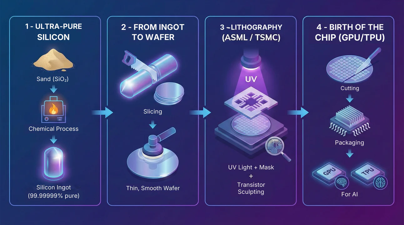
Phase 1: Raw silicon → chip (GPU, TPU, etc.)
1 - Ultra-pure silicon
It all starts with silicon (which is why it’s called “Silicon Valley”, by the way). But why silicon? Because it’s an abundant and unique semiconductor: unlike metals (which always conduct) or insulators (which always block), it lets you control exactly when electricity flows and when it doesn’t. That ability to “switch on and off” is the physical foundation for creating 0’s and 1’s.
To get there, sands rich in silicon dioxide (SiO₂) go through chemical processes at high temperatures to remove impurities. The result is silicon with absurd purity (like 99.9999% or more), formed into big cylindrical ingots.
2 - From ingot to wafer
Those ingots are “sliced” into very thin discs (called “wafers”) with high-precision saws, and polished until they’re smooth at almost the atomic level, because any imperfection turns into an electrical problem later.
3 - Lithography
Here comes the famous process of lithography, the most complex engineering humanity has ever done. It’s like “printing” at the nanometer scale (many orders of magnitude smaller than a human hair), and it depends on machines made by just one company (ASML, from the Netherlands), with the process mostly carried out by TSMC in Taiwan. The process uses ultraviolet light that passes through a mask with the circuit design and “burns” a pattern into a material. It’s like drawing the map of an entire city on the head of a pin. Layer by layer, chemical baths remove what the light touched (or didn’t touch), carving billions of transistors into a ridiculously precise geometry.
4 - The birth of the chip (GPU/TPU)
When all the lithography, doping (injecting atoms of other elements to control how the silicon conducts electricity) and metallization (connecting the transistors with thin layers of copper or aluminum, forming the wires of the circuit) are done, the whole wafer is covered by a “matrix” of tiny chips (called “dies”). Ultra-precise cutting machines slice the wafer into hundreds or thousands of these little squares. Each chip is then tested and packaged (that black/silver case with pins or contacts underneath). Some become CPUs, others GPUs, others TPUs, but they were all born right there, from the same silicon pizza.
For AI, the king is the GPU (or the TPU).
Phase 2: Transistors → logic gates → bits
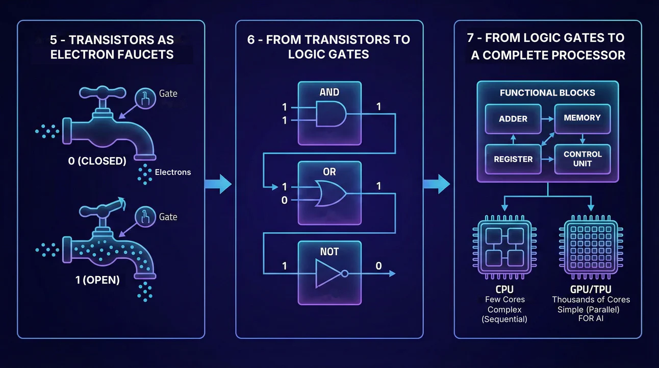
5 - Transistors as electron faucets
After the wafer is cut into lots of chips, each of those little squares already comes with billions of transistors “drawn” by the lithography and wired together in very specific patterns. At the most basic level, a transistor is just a component that controls whether electric current flows between two points. It has a “gate” that, when it receives a certain voltage, changes state: it can let electrons through (like an open faucet), representing the binary value 1; or block them (faucet closed), representing the binary value 0.
6 - From transistors to logic gates
If you connect several transistors in a smart way, you can build blocks that implement simple logical rules: AND (outputs 1 only if all inputs are 1), OR (outputs 1 if at least one input is 1), NOT (flips the signal). These little blocks are the logic gates. They’re so fundamental that every digital operation, no matter how sophisticated it looks, is a gigantic combination of these super simple “little pieces”.
7 - From logic gates to a complete processor
When you connect hundreds, thousands, millions of logic gates, more sophisticated blocks appear: adders that do arithmetic, comparators, counters, registers that hold values temporarily, memory banks that store thousands or billions of bits, and the control unit that decides which operation to run on each clock cycle. In the end, an entire CPU or GPU is a giant castle built on this foundation: transistors → logic gates → functional blocks → processor.
CPUs are perfect for complex sequential tasks, like running an operating system, opening files, making complicated decisions, but when you need to do the same simple operation (like multiplying two numbers) billions of times, the CPU is inefficient. CPUs have a few powerful cores (~8-32), while GPUs have thousands of simple cores (10,000+). It’s like having a math PhD solving 10 thousand simple addition problems: they’re overqualified and way too slow for that kind of work. That’s why we use GPUs (or TPUs).
Taking specialization even further, companies like Google created TPUs (Tensor Processing Units), chips designed exclusively for AI operations. While GPUs are generalists (good for games, rendering, AI), TPUs are highly specialized in one thing: matrix multiplication for deep learning, but they do it with absurd energy efficiency.
Phase 3: Processor clock → sequence of operations
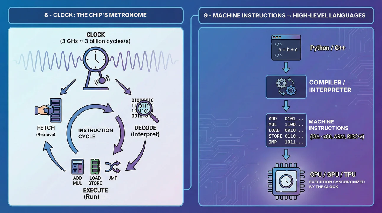
8 - Clock: the chip’s metronome
Inside the chip (CPU, GPU, TPU, etc.) there’s an internal “clock” that sets the rhythm of everything. When you see something like 3 GHz, that means the processor does about 3 billion cycles per second. Each cycle is a “tick”: the pulse that coordinates when electrical signals should be read, propagated and updated. Without that clock, each part of the chip would work on a different timing and chaos would reign.
On each cycle, the processor does nothing “magical”, it just takes one more step: first it fetches from memory the next instruction (fetch), then it decodes the bit pattern to understand what it means (decode) and, finally, it executes the requested operation (execute), like adding two numbers, multiplying, comparing values, loading data from RAM, writing results, jumping to another part of the code and so on. All of that is just electrons running along metal tracks and transistors switching on and off, synchronized to the millimeter by the clock.
In practice, modern processors do several things in parallel on each cycle, but this “one step per tick” view works well as a mental model.
9 - Machine instructions → high-level languages
What the processor really understands are machine instructions, defined by an instruction set architecture (ISA) like x86, ARM or RISC-V. Each instruction is a bit pattern that can be seen with friendlier names like ADD, MUL (multiply), LOAD (load from memory), STORE, JMP (jump), etc.
Programming directly in those instructions would be insane for something the size of a modern AI model, so we write in high-level programming languages (closer to human language), like C++ or Python. Compilers and interpreters play the “midfielder”: they translate the code you write into machine commands and calls to super-optimized libraries (like cuBLAS, cuDNN, MKL…), which in turn become a sequence of ADD, MUL, LOAD, STORE running at the pace of the clock.
Phase 4: Data in memory → programming frameworks for AI
10 - RAM: the processor’s scratchpad
When you run a program (AI or not), the processor doesn’t work alone. It needs a place to keep temporary data while it does the math: RAM. RAM is like a gigantic spreadsheet where each “cell” has a unique address and can hold a few bytes. When the processor needs to add two numbers, it first uses LOAD to fetch those numbers from RAM, brings them into the chip (into the registers, those tiny ultra-fast spaces inside the GPU/CPU), does the math, and uses STORE to save the result back. This back-and-forth between processor and memory happens trillions of times per second.
11 - RAM vs VRAM
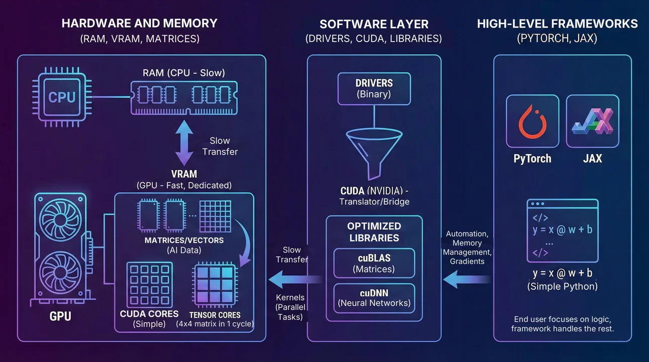
Here comes a crucial distinction: regular RAM (where the CPU works) and VRAM (Video RAM, the RAM dedicated inside the GPU itself). Moving data between RAM and VRAM is relatively slow, so AI models try to keep everything in VRAM as much as possible. When you load a 70-billion-parameter AI model, you’re basically filling the VRAM of several GPUs with those numbers, organized in giant matrices.
12 - Vectors and matrices
For AI, you don’t work with one or two numbers. You work with millions or billions of numbers, organized in vectors and matrices. For example, a 1000×1000 matrix has 1 million numbers stored sequentially in VRAM. The processor doesn’t “see” that as a nice table, it sees a continuous block of memory addresses, but optimized libraries (like NVIDIA’s cuBLAS or PyTorch) know exactly how to navigate those addresses, load whole chunks of data at once (using cache and memory bandwidth), and spread the work across thousands of GPU cores.
GPUs were originally created for 3D graphics in games, where you need to compute the color of millions of pixels at the same time. For that, NVIDIA (and others) built chips with thousands of small, “dumb” cores: each one only knows how to do simple operations (add, multiply), but they all work in parallel. A modern GPU can have tens of thousands of cores crunching numbers at the same time.
For AI, the most important thing is one specific operation: matrix multiplication. It’s the basis of everything neural networks do. And precisely because of that, NVIDIA created even more powerful specialized hardware inside modern GPUs: NVIDIA’s Tensor Cores or Google’s MXUs. They’re dedicated processing units that do matrix multiplication absurdly faster than the regular cores (CUDA cores). While a CUDA core does one multiplication at a time, a Tensor Core can do an entire 4×4 (or larger) matrix multiplication in a single clock cycle. It’s as if, instead of adding 1+1, then 2+2, then 3+3… you could add 100 pairs of numbers at once. That speeds up training and inference of AI models by up to 10x or more.
13 - Drivers and Kernels (CUDA)
The chip (GPU) is a brute-force monster, but it doesn’t speak English or Python. It speaks binary. For your code to be able to boss the GPU around, there’s a critical layer of software: drivers and low-level libraries. For that, in 2006, NVIDIA launched CUDA (Compute Unified Device Architecture), a platform that lets you program the GPU to do any kind of parallel computation, not just graphics.
CUDA is basically an extension of the C/C++ language with special commands to control the GPU. You write code saying “take this matrix and spread the work across all available cores”, and CUDA provides “kernels”, which are small super-optimized functions written specifically to run in parallel on the GPU, and takes care of the orchestration of all of that. When you ask for a matrix multiplication in Python, CUDA translates it and assigns thousands of GPU cores to solve little pieces of the problem at the same time. It’s the translator that turns your logical intention into electrical signals in the transistors.
Most AI scientists don’t write CUDA directly (it’s complex). NVIDIA created fundamental libraries written in CUDA that do specific operations in an ultra-optimized way: cuBLAS (for matrix multiplication), cuDNN (for neural network operations like convolutions), cuSPARSE (for sparse matrices), TensorRT (for fast inference). These libraries are the result of years of engineering: NVIDIA engineers optimize every detail of how to lay out data in memory, how many threads to use per block, how to minimize transfers between GPU and RAM. They’re the “engine” that makes everything run fast.
14 - Frameworks for AI (PyTorch and JAX)
Even using cuBLAS and cuDNN, building a neural network would still be a lot of work. That’s where frameworks like PyTorch (from Meta) and JAX (from Google) come in. They’re like “high-level programming languages” specialized in AI:
PyTorch: You write Python code that looks super simple, like y = x @ weights + bias. Under the hood, PyTorch translates that into calls to the CUDA libraries (cuBLAS, cuDNN). It also manages memory automatically, computes gradients (derivatives) for you during training (autograd), and lets you move tensors (multidimensional matrices) between CPU and GPU with a single command.
JAX: Similar to PyTorch, but with a different focus. JAX compiles your Python code into XLA (Accelerated Linear Algebra), a compiler that optimizes the operations even further before they turn into CUDA. JAX is also famous for making it easy to parallelize across multiple GPUs/TPUs and for allowing automatic differentiation of pretty much any function.
When you write a command to do a matrix multiplication, like torch.matmul(A, B) or jax.numpy.matmul(A, B), you’re not thinking about threads, blocks, or core synchronization. The framework takes care of that: it calls cuBLAS, which calls optimized CUDA kernels, which spread the work across thousands of GPU cores. It’s automation on top of automation on top of automation.
Phase 5: The neural network
15 - Defining a neural network
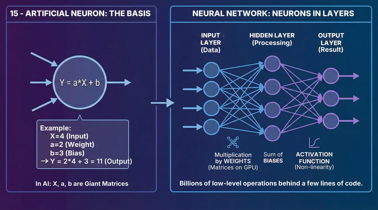
A generative AI model, like ChatGPT, Gemini, Claude, etc., is built from a neural network. A neural network is a computational graph made of artificial neurons, which are nothing more than small pieces of code that apply a mathematical function to the values they receive. Example: take the classic linear function “Y = a*X + b” - in this case, the neuron’s input would be “X”, which is multiplied by a weight “a”, then a constant value “b” is added, and the neuron’s output would be “Y”. So, if a = 2, b = 3, and we have an input X = 4, the result would be Y = 2*4 + 3 -> Y = 11. The difference in an AI model is that those values aren’t single numbers, but giant matrices of numbers, which get multiplied by the “weights” (the “a” in the equation), added to a “bias” (the “b” in the equation), and that result is passed on to the neuron in the next layer.
Yes, these neurons are organized in layers. Data comes in one side (input layer), goes through dozens of intermediate layers (hidden layers) and comes out the other side (output layer). In each layer, the input data is multiplied by the weights (that matrix multiplication the GPU loves to do!), added to the biases, and then goes through an “activation function” (a mathematical operation that introduces non-linearity, and decides whether that neuron should “fire” or not). In code, this looks simple, like 20 lines in PyTorch or JAX, but when you hit run, the framework blows that up into billions of low-level operations.
16 - The Transformer architecture
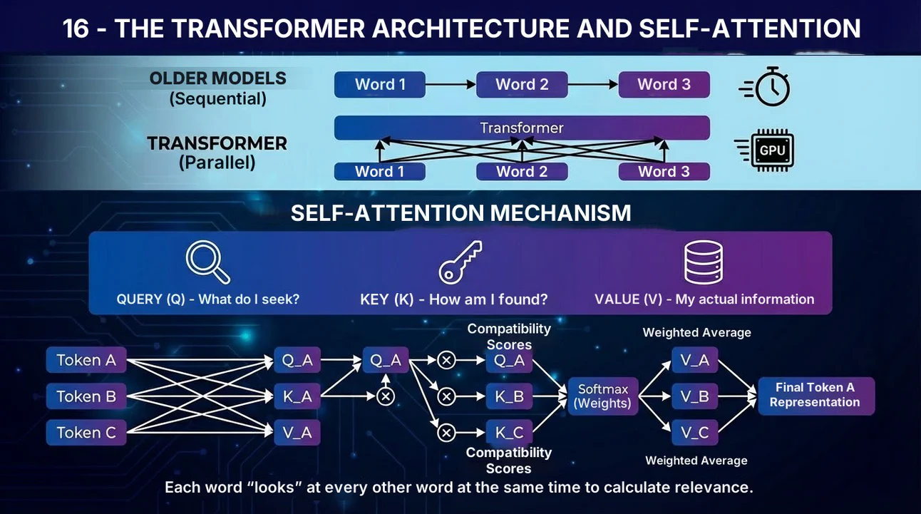
The Transformer architecture was the revolution that made the leap to today’s AIs possible. It’s a specific way of organizing those layers of neurons and activation functions. Unlike the older models that read a sentence word by word, sequentially (like we read), it takes in the whole sequence at once, which fits perfectly with the massive parallelism of GPUs.
The secret is the self-attention mechanism: imagine that each word in the sentence can “look” at all the other words at the same time and mathematically calculate how relevant they are to each other. In practice, self-attention works like a search in a giant dictionary. Each token (word) generates three different versions of itself through multiplications by different matrices:
- Query: Represents “what this token is looking for” in the other words.
- Key: Represents “how this token can be found” by others.
- Value: Holds the actual information this token is going to contribute.
The process works like this:
Each token takes its query and multiplies it by the keys of all the other tokens (including itself). That generates a compatibility score: “how relevant is this word to me?”.
Those scores become attention weights (using softmax, a mathematical function that turns any list of numbers into probabilities that add up to 100%, for example: [2.1, 1.0, 0.3] becomes [70%, 25%, 5%]).
Finally, those weights are used to take a weighted average of the values of all the tokens. Tokens with a high weight contribute a lot; tokens with a low weight contribute little.
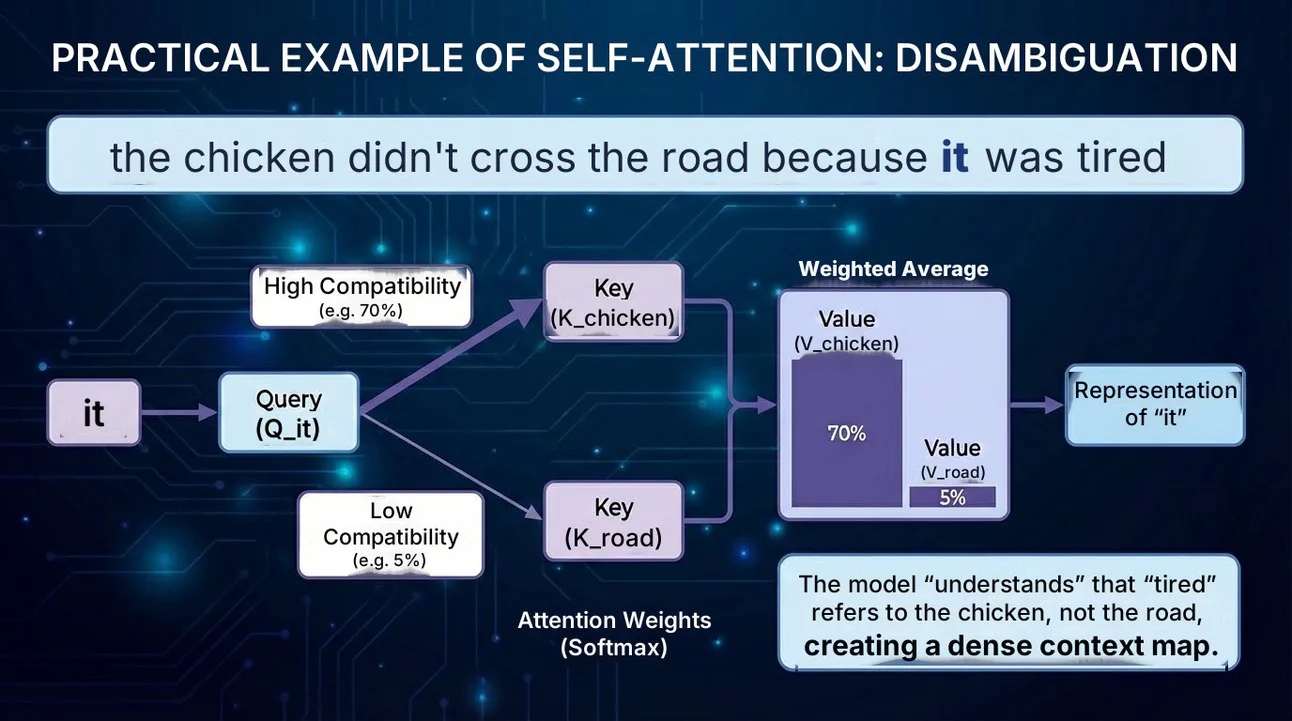
This creates a dense map where each word knows its relationship with all the others, regardless of distance in the sentence, allowing the model to handle complex disambiguation, like knowing that in the sentence “the chicken didn’t cross the road because it was tired”, the word “tired” refers to the “chicken” and not to the “road”, creating a dense map of context and meaning that earlier models couldn’t form.
In practice, in that sentence, when the model processes the token “it”:
- The query of “it” is multiplied by the keys of all the words
- The key of “chicken” has high compatibility → gets a high weight (say, 70%)
- The key of “road” has low compatibility → gets a low weight (say, 5%)
- The value of “chicken” contributes 70% to the final representation of “it”
So, the model understands that “tired” refers to the “chicken”, not to the “road”.
Phase 6: Data, tokenization and model training
17 - The training dataset
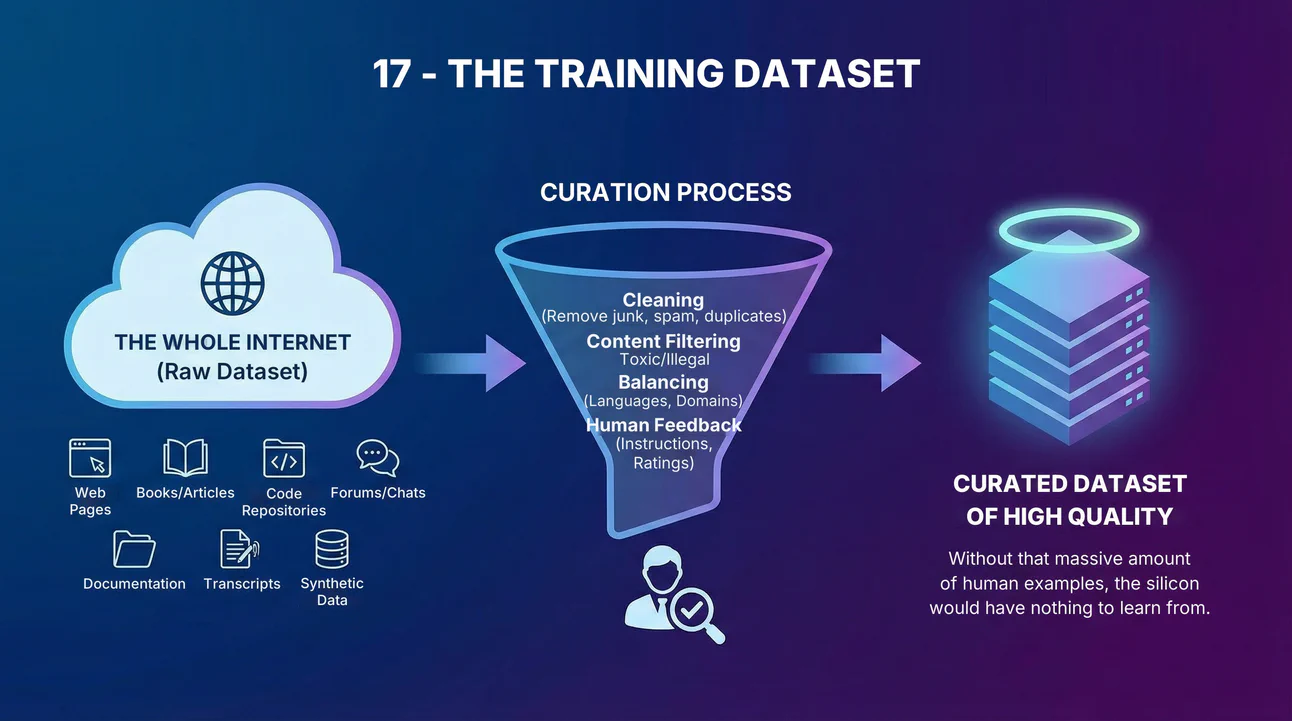
These AI models need LOTS of data to learn, REALLY A LOT, like, the WHOLE internet. Web pages, books, articles, code repositories, forums, chats, technical documentation, transcripts, synthetic data generated by other models… Before it reaches the GPU, this material goes through a heavy curation stage: cleaning (removing junk, spam, duplicates), filtering toxic or illegal content, balancing languages and domains (how much technical text vs. casual conversation vs. news), and, in more aligned models, special datasets of instructions and human feedback also come in (people rating better and worse answers). Without that massive amount of human examples, the silicon would have nothing to learn from.
18 - Tokenization: turning text into numbers
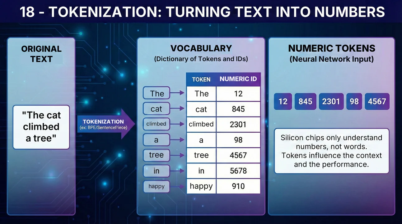
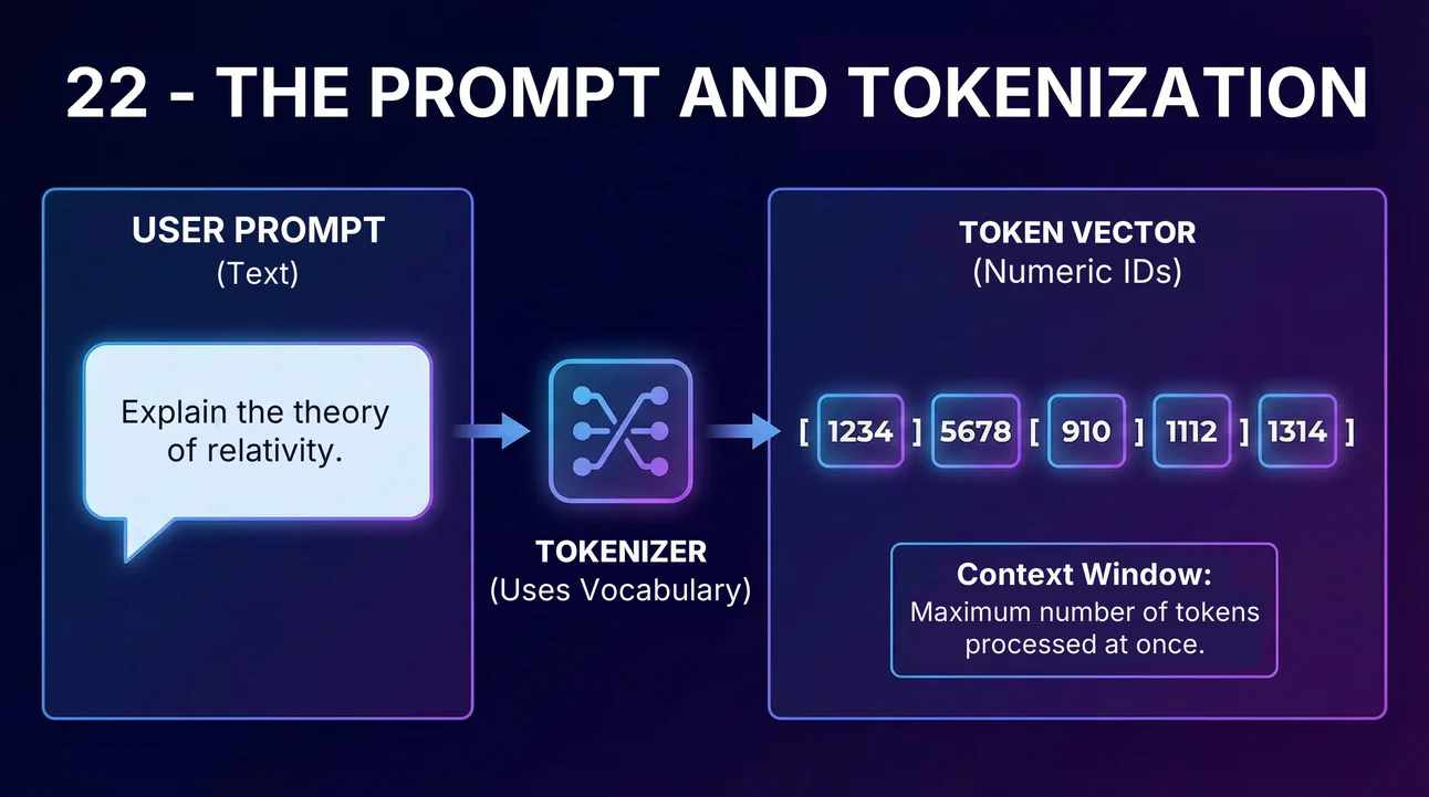
Before any training happens, there’s a problem: silicon chips don’t know what the letter “A” or the word “house” is, they only understand numbers. This is where the tokenization process comes in. What it does is, basically, break that gigantic text from the dataset into smaller pieces called “tokens” and assign a unique number to each one. A token can be a whole word (“dog” → 1234), a piece of a word (“un” + “happy” → 5678, 910), or even individual characters, all depending on the language and on the amount and frequency of that data in the dataset.
Modern models use algorithms like BPE (Byte Pair Encoding) or SentencePiece, which analyze the whole dataset and figure out which combinations of characters show up most often, creating an optimized “vocabulary”. For example, the word “unhappy” might be common enough to be a single token, or it might be broken into smaller pieces (“un” and “happy”) if it’s rarer. In the end, you have a dictionary with 50 thousand, 100 thousand or even 200 thousand possible tokens, each with a numeric ID.
This vocabulary is fixed once it’s created. When the model is trained or used, any text that comes in is immediately converted to numbers using that same table. Those numbers are what actually enter the neural network:
[The, cat, climbed, the, tree] becomes something like [12, 845, 2301, 98, 4567].
Why does this matter? Because tokens influence everything: how many tokens a model can process at once (the “context”), how many mathematical operations will be needed, and even how the model “thinks”. Rare words broken into many tokens are harder for the model to understand. Depending on the tokenizer, languages with non-Latin scripts (Chinese, Arabic, Japanese) will need more tokens to express the same thing, which can affect performance.
19 - Embeddings: the semantic representations
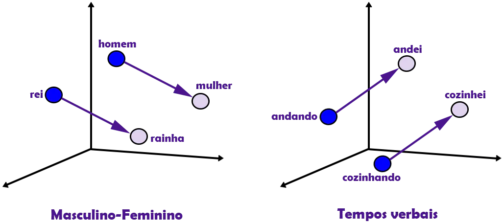
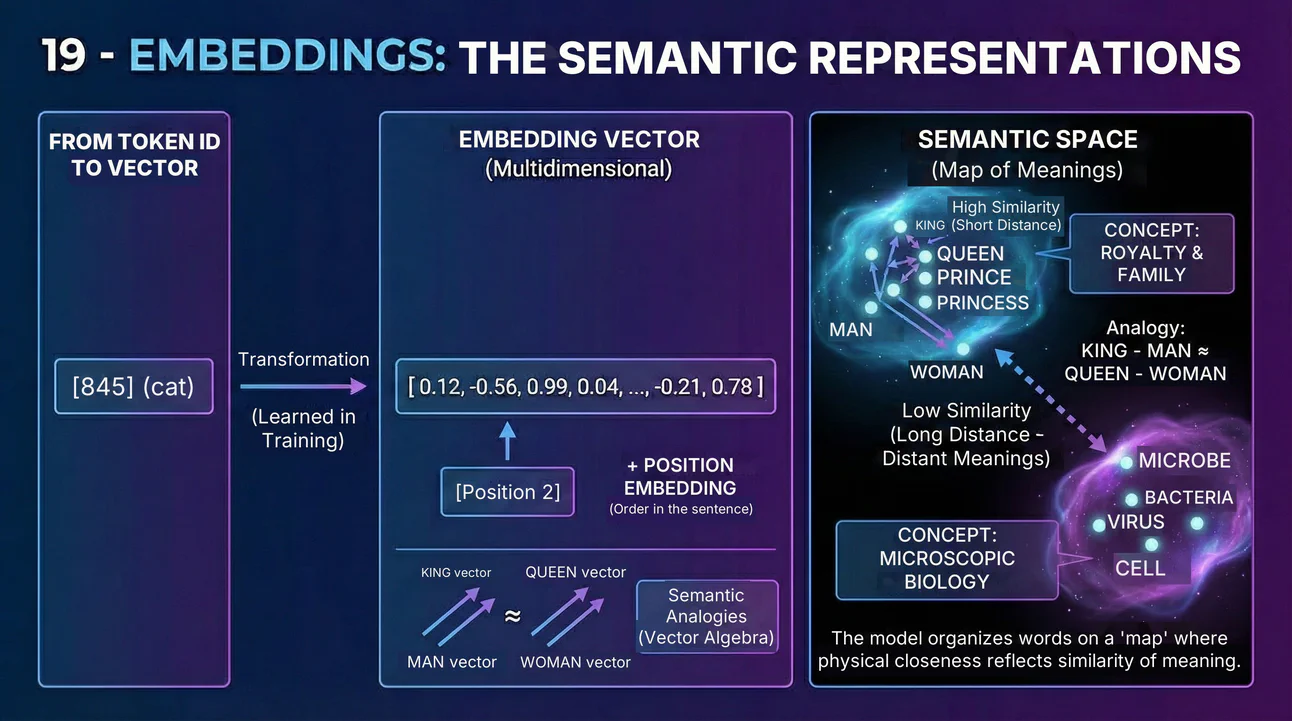
But the ID number alone isn’t enough, the model needs to understand the meaning of the word. That’s where the embedding comes in: each token ID is turned into a long vector of numbers, like [0.12, -0.56, 0.99, …], which places that word in a multidimensional mathematical space, and serves as a semantic representation of that word (of that token, actually) in relation to all the others extracted in tokenization.
Words with similar meanings (like “king” and “queen”) will have vectors that are mathematically close in that space; words that don’t have much to do with each other (like “king” and “microbe”) are far apart mathematically. The cool part is that these embeddings capture subtle relationships: the vector difference between “king” and “queen” is similar to the difference between “man” and “woman”, creating a kind of “semantic algebra”.
These embeddings aren’t fixed from the start. They begin with random values and are learned during training, being adjusted along with all the other weights of the neural network. As the model sees billions of text examples, it figures out on its own that “cat” and “feline” should be close, that “Paris” and “France” have a geographic relationship, and so on. It’s one of the most fascinating aspects of deep learning: the model discovers these complex semantic relationships just by trying to predict the next word correctly.
On top of each token’s embedding, the model adds a positional embedding, which says where in the sentence that token sits. Without it, it would see the sentence as a bag of words with no order.
20 - Training the neural network
This is where everything we’ve seen so far comes together. To create a model like GPT or Gemini, we don’t use one GPU, but tens of thousands of them connected in gigantic clusters (supercomputers), running day and night for months. The training process of a neural network is a gigantic cycle of trial and error:
Forward pass: The still “dumb” model (just the “shell” of the neural network structure, with weights and biases initially filled with random values, including the embeddings) tries to guess the next word (actually, the next “token”) of a text from the dataset. The data goes in through the input layer, passes through all the intermediate layers with their matrix multiplications, and reaches the output of the last layer.
It gets it badly wrong. Based on that, it calculates how big the error was through a “loss function”, a mathematical equation that compares the model’s prediction with the correct answer. The lower the value of the loss function, the better the prediction.
Backpropagation: This is where the math gets heavy. The algorithm computes the gradients (basically, the mathematical derivatives that show in which direction and by how much each weight contributed to the error). It’s like figuring out: “if I had increased this specific weight by 0.001, would the error have gone down or up?”. This calculation uses the chain rule from calculus and walks through the network backwards, layer by layer.
Optimization: With the gradients in hand, an optimizer algorithm (like Adam, SGD or AdamW) decides exactly how much to adjust each weight. Backpropagation says “adjust up” or “adjust down”, but the optimizer decides the size of the step. It takes into account not only the current gradient, but also a history of past gradients to make smarter, more stable adjustments.
Weight update: Billions of weights (including the embeddings from step 19) are adjusted slightly: values like 0.452 become 0.453, or -1.239 becomes -1.238, etc. It seems like very little, but it’s billions of adjustments happening simultaneously.
This is where matrix multiplication happens at industrial scale. It runs in gigantic loops, for months, on clusters with thousands of interconnected GPUs. Each GPU is doing trillions of matrix multiplications per second. The energy consumption is absurd: training a large model can cost millions of dollars in electricity alone.
When training ends and the error is acceptable, the process stops. What’s left is a giant static file (tens or hundreds of GB) full of nothing but decimal numbers. That file contains the final parameters (weights, biases and embeddings), those billions of numbers (like 0.452, -1.239, 0.001…) that were adjusted to the millimeter during months of training and represent the strength of the connections between the artificial neurons. If a weight is high, the connection is strong; if it’s negative, it’s inhibitory.
The “knowledge” of an AI model is nothing more than the fossilized result of those almost infinite back-and-forths to adjust the values of the weights and biases, and it’s encoded in the exact combination of those billions of numbers. That’s precisely why, if you stopped collecting training data for the model in December 2025, it won’t have the slightest idea if you ask about some fact that happened in January 2026. The knowledge is literally “frozen” in those numbers (though, in production, modern systems can use tools like web search to access up-to-date information).
In general, you can split this step 20 into two big phases: pre-training and post-training:
Pre-training: the model learns, from all that data, only to predict the next token, adjusting weights to get better and better at that task. Something like a super autocorrect on your phone, suggesting the most likely next word.
Post-training: this is where it gets its “assistant personality”: supervised fine-tuning with instructions comes in (people writing examples of questions and good answers) and, often, techniques like RLHF (Reinforcement Learning from Human Feedback) or DPO (Direct Preference Optimization, a more direct way of training from human preferences), where humans rate better and worse answers and the model is adjusted to follow instructions, be more helpful, polite and safe.
In the end, the weights file you load on the GPU is the combined result of those two stages: first it becomes a great “text predictor”, then it’s polished to behave like an assistant that talks to you.
Phase 7: Inference (the model generating an answer)
21 - Loading the model into memory
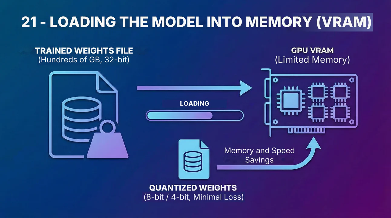
That giant file of trained weights has to be loaded into the GPU’s VRAM to be used. That can be hundreds of gigabytes, and very large models don’t even fit on a single GPU, so they’re spread across dozens of GPUs working together. Each GPU holds a slice of the weights and syncs the results with the others.
To make giant models fit on fewer GPUs or run faster, a technique called “quantization” is often used. It means reducing the precision of the weights (for example, from 32 bits to 8 or even 4 bits per number). That drastically shrinks the size of the model in memory, with minimal loss of quality in the answer.
22 - The prompt
When we talk about a language model like GPT, Gemini or Claude, your prompt is the question/request you send to the model. Let’s say you want to ask it: “Explain the theory of relativity.”. But remember that the computer doesn’t understand words, only numbers. So your prompt uses that same tokenization vocabulary created in step 18 to convert your prompt into numeric tokens. That way, your prompt becomes a vector of IDs, like [1234, 5678, 910, 1112, 1314].
It’s also worth saying that the model can only see a maximum number of tokens at once, which is called its “context window”. Your prompt + what it has already generated can’t go over that limit, or else it has to truncate or discard older parts of the conversation.
23 - The inference process in the neural network
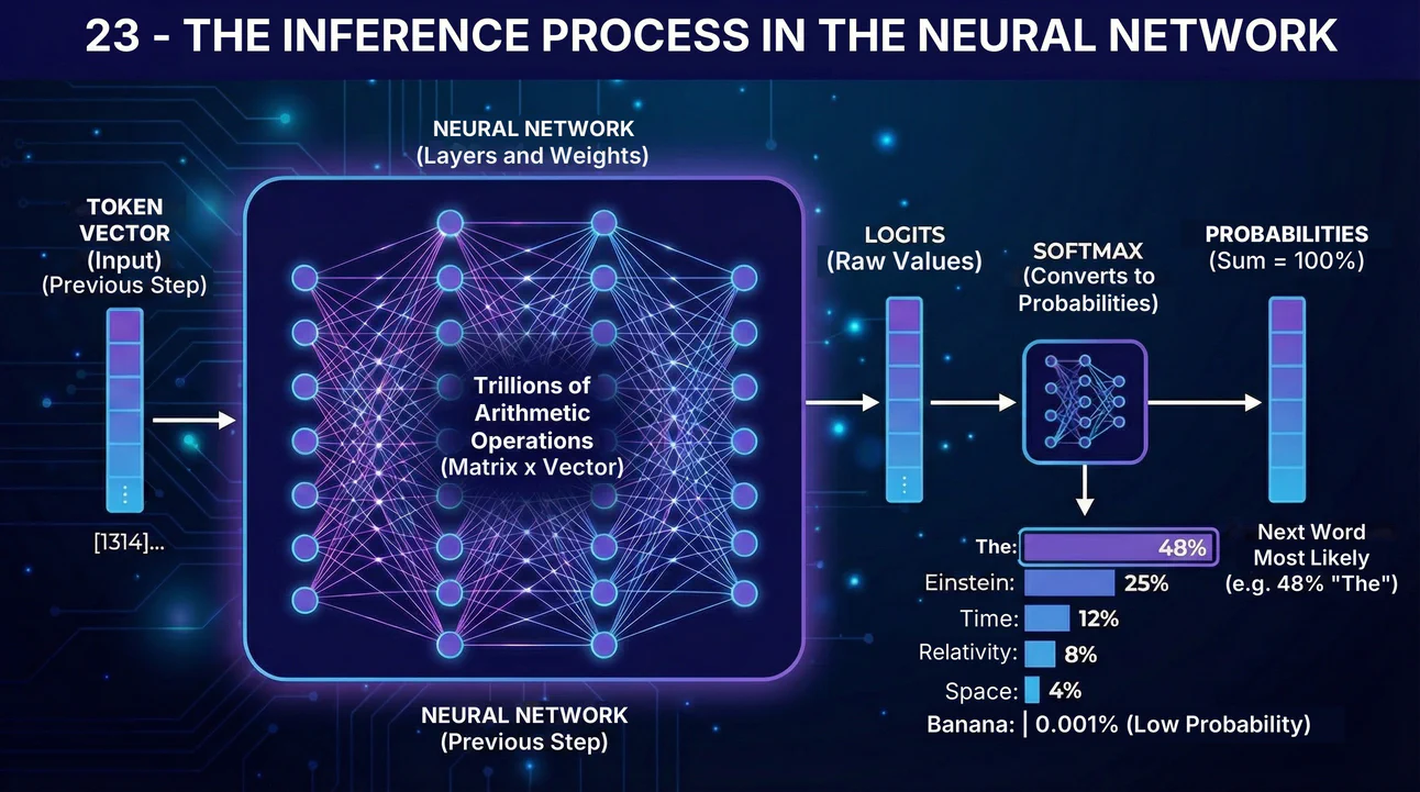
This is where the magic happens and all that silicon from Phase 1 goes to work. Your prompt’s vector enters the first layer of the neural network. Then the GPUs spring into action, taking that vector and multiplying it by the gigantic weight matrices (step 20), layer after layer, at the pace of the clock (step 8). That’s trillions of arithmetic operations happening in milliseconds. The heat generated in the GPUs is dissipated by advanced cooling systems, while the electrons run through the transistors.
After going through all the layers, what comes out at the last end are called “logits”, which are a vector the size of the full vocabulary with raw values for each possible token in the vocabulary. Those logits then go through that mathematical function, “softmax”, which converts them into a giant list of probabilities (where all of them add up to 100%).
The model looks at your prompt ("Explain the theory of relativity.") and at everything it has generated so far, and calculates: “Given this input, what’s the probability that each of the 100,000 tokens in my vocabulary is the next correct word?”.
It might calculate that there’s a 48% chance the next token is “The”, 25% that it’s “Einstein”, 0.001% that it’s “banana”, etc. An algorithm will pick one of those words based on these probabilities (usually the most likely one, but sometimes varying a little, according to some parameters like “temperature”, “Top-P”, “Top-K”, etc., to be more creative or to avoid certain tokens).
Since the model picks based on probability, sometimes it may choose a path that’s statistically possible but factually wrong. That’s where hallucinations are born: the model being too “creative” or relying on wrong patterns from the training data.
Great, let’s say the model has chosen the first token of the answer: “594” in the dictionary, corresponding to the word “The”. But the process isn’t over. Now, that token “The” is appended to your original prompt. The new input for the model is now: “Explain the theory of relativity. The…”.
The whole process of steps 22 and 23 repeats. The GPU runs all the calculations again with the new extended input to predict the second token. And then the third. The model does this over and over, word by word (token by token), until it decides the answer is complete and generates a special “end of text” token. As you’ve certainly experienced, the answer tokens are sent to the user one by one via streaming, without having to wait for the final token to send everything at once.
In practice, to avoid redoing all the math from scratch on every token, the model caches certain intermediate information (the famous attention “KV caches”). That way, each step reuses what was already computed and only does the new calculations needed.
Worth mentioning that during this inference process (when you use the chat), the model does NOT learn new things. Nothing you type changes the model’s weights at that moment (unless the company uses your data in a future training run).
Conclusion
And that’s how, starting with purified sand and ending with trillions of matrix multiplications per second, a question on your screen turns into an intelligent answer.
The most fascinating part is that none of this is magic. Every step is purely mechanical: electrons running along copper tracks, transistors switching on and off, numbers being added and multiplied. There’s no hidden “soul” in the code, there’s no moment where something supernatural happens.
And yet, when you stack billions of these simple operations, organized the right way on this sand, fed with enough data, something surprising emerges: patterns that look like understanding, answers that look like reasoning, text that looks like thought.
The next time an AI answers you, you’re not talking to an alien intelligence or an artificial consciousness. You’re watching a very concrete chain in action: sand → ultra-pure silicon → transistors → processors and GPUs → massive matrix multiplications → text on your screen. All of it guided by billions of weights adjusted by trial and error over months of training.
It’s proof that enough complexity, even when born from simple rules, can imitate (and sometimes surpass) abilities we considered exclusively human.
From silicon sand to chat. From organized electrons to the text on your screen. That’s how it works.