[TUTORIAL] Pruning and distillation of LLMs: how a 40B model teaches a 20B one, token by token
Published on
This article is going to be a mix of explaining what pruning and distillation are in AI and LLMs, and a tutorial on how to do them, alright?
It all starts with a real pain: running a 40-billion-parameter LLM isn’t for everyone. Its weights alone, in BF16, take up about 80 GB of memory (40 billion × 2 bytes), so it doesn’t even fit whole on an 80 GB GPU, let alone leave room for the conversations.
What if you could cut that model in half and still keep pretty much everything it knows, like its language skills, function calling, etc.?
That’s exactly what I’ve been doing these past few weeks with ALIA-40B, the open model from the Barcelona Supercomputing Center (BSC), where I work as an AI Developer Advocate and Research Engineer. The idea is to turn it into an ALIA-20B with two techniques that go hand in hand: pruning and knowledge distillation (or just “KD” to its friends).
In this post I’m going to open both of them up, including a real training step from the project. And at the end I’ll leave you the step-by-step guide with the frameworks and code we use, from pruning all the way to evaluation.
Shall we?
Why shrink a model instead of training a small one from scratch
It’s a fair question: if I want a 20B model, why not train a 20B model from scratch? The answer is cost, both in time and in money. ALIA-40B was pre-trained on 9.37 trillion tokens, and repeating that for every model size would burn a mountain of GPU hours.
NVIDIA showed a shortcut in 2024, with the Minitron family. In the paper Compact Language Models via Pruning and Knowledge Distillation, they took the Nemotron-4 15B model and managed to create 8B and 4B models from it using less than 3% of the original training data, that is, up to 40 times fewer tokens per model than training from scratch, and up to 16% more on MMLU than the same models trained from scratch. Later they repeated the recipe with Llama 3.1 8B (which became a 4B) and with Mistral NeMo 12B (which became Mistral-NeMo-Minitron-8B), in a second paper.
The recipe has two parts, and it’s worth defining both right away:
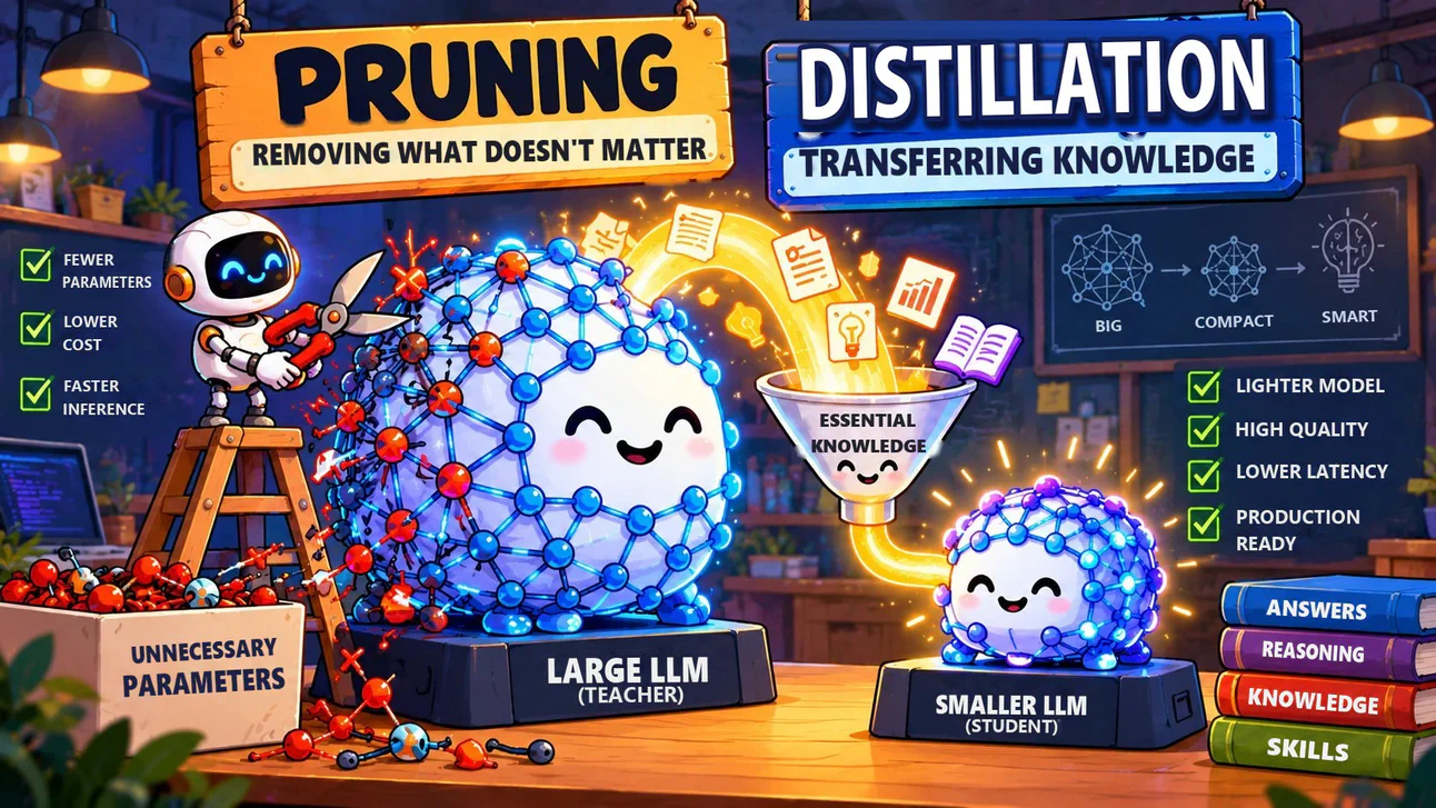
- “Pruning” means cutting whole parts out of an already trained model, like layers, neurons and attention heads, choosing the ones it misses least. The model gets smaller instantly, but it comes out kind of groggy.
- Distillation (KD) means training the smaller model, the student, to imitate the predictions of the big model, the teacher. It’s what fixes the damage from the pruning.
Pruning is just like pruning a tree that’s too big for your backyard: you cut the branches that bear the least fruit, but the trunk and roots are still there (the student inherits the teacher’s weights, so it doesn’t start from scratch). Distillation, on the other hand, is like a kitchen apprentice who, instead of memorizing only the final dish, stands next to the chef watching every decision, including the spices the chef used and the ones they ALMOST used.
(And if you’ve read my quantization tutorial, you can think of it like this: quantization stores each of the model’s numbers with fewer bits, while pruning reduces how many numbers there are. You can even combine the two.)
The project: from ALIA-40B to ALIA-20B
The original ALIA-40B is an open model (Apache 2.0 license) from BSC, trained on 35 European languages and 92 programming languages, with Spanish, Catalan, Galician and Basque counting double in the data mix (it comes from a Spanish research center, after all). The teacher I’m using in this project is an improved version with more skills: ALIA-40b-fc-2607.
But it has a problem. Even though it writes really well in those languages, it sometimes struggles with comprehension, following instructions (instruction following), calling functions (function calling) and very long contexts. In other words, it’s a B-minus teacher, not an A-plus one.
That’s why my goal is ambitious: to get to an ALIA-20B that’s exceptional at following instructions, calling tools, working as an agent in long conversations (from 64,000 to 128,000 tokens) and in the Iberian languages. In practice, that means beating the teacher itself at pretty much everything.
The road has four stages: pruning, distillation, SFT with DPO and, at the end, reinforcement learning (RL). Distillation is the stage the project is in right now, and it’s the one I’m going to go through in detail in this article.
Notice that the project has two teachers, each with a different job:
ALIA-40b-fc-2607 itself teaches what it does best, which is knowledge and fluency in the Iberian languages, and it teaches through distillation, passing on the probabilities it gives each token (I’ll explain this better in a moment). But, as I said, following instructions, calling tools and acting in long conversations aren’t its strong suit. That’s why I decided to call for help: Qwen3.8-27B, which is fantastic at those specific skills and was chosen to teach them. Going back to the kitchen apprentice analogy from above: the house chef teaches the seasoning, and a guest chef teaches how to handle the orders and use the fancy new knife.
And why that chef in particular? Before any benchmark, the chosen teacher’s license had to allow training and publishing the final model, and here the terms of use of OpenAI and Anthropic forbid using their models’ outputs to train a competing model, so GPT and Claude are out right off the bat (and a closed model, in general, only runs through its owner’s API). Qwen3.8-27B is Apache 2.0.
On top of that, among the ones that pass those filters, it was the one that did best in my tests. In one of the internal benchmarks I created for BSC, with 2,862 questions from Catalan proficiency exams, Qwen gets 81.6% right, against 80.0% for Google’s Gemma 4 31B (one of the models ALIA-20B has to beat). So far, it’s almost a tie with Gemma. But when the models can consult Catalan spelling, grammar and synonym tools during the exam, Qwen goes up to 87.2% and Gemma to 83.1%. And using tools in the middle of a conversation is exactly one of the things it’s going to teach.
Then, in the project’s own tests, it beat ALIA-40B by 23 to 31 points on IFEval, a test of following instructions (things like “answer in three paragraphs without using a single comma”), in all six languages. And on RULER, a long-context test I explain further down, it scores 96 points (out of a possible 100) across contexts from 16,000 to 128,000 tokens, while ALIA-40B drops from 79 to 49.
Of course, there are caveats. Without its reasoning mode, Qwen drops to 70.8% on the Catalan exam and falls behind Gemma (73.2%), so, in its role as teacher, it will always generate with reasoning on. And it writes worse than ALIA in Catalan, Galician and Basque, but I’ll tell you about that at the end, along with what I did about it.
So, if you’re going to do something similar for another language, the logic is this: first you filter by license and terms of use, and only then do you test the ones left in your language and on the skills you want to teach.
Phase 1 - Pruning: removing what the model uses least
NVIDIA’s Minitron framework is really fantastic. It’s what takes care of this pruning and shrinks the model from 40B to 20B, but how does it decide what to cut? Easy. It runs the teacher model (in my case, the 40B) on a bunch of calibration texts and measures the magnitude of the activations of each piece of the neural network: each neuron, each attention head, each channel of the main dimension and each layer. Then the pieces that barely “light up” are the first to go, and the weights of what’s left are sliced and copied as they are.
In the project, the calibration used 1,024 windows of 4,096 tokens (about 4.2 million tokens) mixing Spanish, Catalan, Galician, Basque, Portuguese, English, code and math, with Galician and Basque weighing more than they do in training. The logic is simple: if the calibration barely saw any Galician or Basque content, the neurons that work for those languages could end up being thrown out. The whole pruning took about 10 minutes on a single node, no sweat.
And what can you cut? In a Transformer like ALIA (which follows the Llama architecture), there are four axes:
- Depth (layers): ALIA-40B has 48 stacked blocks, like the floors of a building. Cutting depth means removing entire floors.
- Model dimension (hidden): each token travels between layers as a vector of 8,192 numbers. That’s the width of the hallway that ALL of the model’s information goes through.
- FFN: each block has a feed-forward layer with 24,576 neurons, where a good chunk of what the model “knows” lives.
- Attention heads: 64 per block, each one looking at the text in a different way.
To get to 20B, you can combine those cuts in lots of ways, and Minitron doesn’t tell you which is best. So what’s recommended is something like an A/B test: prune several ~20B shapes (named A, C, E, F and G) plus four “diagnostics” that cut a single axis, and measure how much each of those versions loses, on text in every language (or on whatever skills we want to test):
The loss here is the NLL (Negative Log-Likelihood, the same cross-entropy from my post about loss functions), in nats per token. A “nat” is the unit of information you get when the math uses the natural logarithm (ln, base e ≈ 2.718). The idea is the same as the bit, which uses base-2 logarithms: 1 nat ≈ 1.44 bits. The name comes from “natural unit”. In the NLL, each token costs −ln(p), where p is the probability the model gave the token that actually came next in the text. If the model gave the right token 100%, the loss is 0 nats; with 50% it’s 0.69, with 10% it’s 2.30 and with 1% it’s 4.61. A blind guess among the 256,000 tokens costs 12.45. So nats per token is the average of that over the whole text, and the lower, the better.
This analysis already shows some really interesting things. In my case with ALIA-40B:
- The most expensive cut is the hidden one. Just going from 8,192 to 6,144 took the loss from 1.76 to 5.73. In pruning candidate C, that cut alone accounted for about 80% of the damage (3.97 of the 4.93 extra nats). That’s what made me test candidate G, which keeps more hidden (7,168) and makes up for it by slimming down the FFN (12,800) and removing 8 layers. It came out 1.93 nats ahead of candidate E, which removes the same layers.
- Removing layers was the cheapest. Cutting from 48 to 44 layers cost only 0.08 nats. The middle layers, between 23 and 30, were the most expendable: skipping one of them costs 0.024 to 0.029 nats. Layer 0, on the other hand, is sacred (without it, the loss goes up 7.7 nats).
- Cutting attention heads hurts the smaller languages more. Going from 64 to 48 heads raised the loss by 1.96 nats in Catalan, 1.52 in Basque and 1.38 in Galician, against 0.55 in Spanish and 0.64 in English.
- The cuts add up, and not in a pretty way. Pruning candidate A combines the head cut with the hidden one and reaches 11.29 nats, almost a random guess (12.45, which is the natural log of 256,000).
But there’s a catch in this chart: the loss before distillation is misleading. Candidate A, which looked practically dead, caught up with C in about 50 KD steps. So what really decided the base candidate was a short distillation race (the ModelOpt documentation itself recommends this: distill each candidate a little before choosing). Each one trained on about 300 million tokens, and candidate G came out ahead on 7 of the 8 validation sets (the six languages, code and math).
Result: the candidate chosen to be my student model was G, with 40 layers, a hidden size of 7,168, an FFN of 12,800 and all 64 heads, for a total of 19.97 billion parameters (it’s the “Candidate G” tab of the axes diagram, up above). In BF16, that’s about 40 GB, which already fits on an 80 GB GPU with plenty of room for the conversations. And after about 2 billion distilled tokens, its loss dropped from 4.52 to 2.00 nats, against the teacher’s 1.76.
Phase 2 - Distillation: the teacher and the student
The idea of distillation is from 2015, from the paper Distilling the Knowledge in a Neural Network, by Geoffrey Hinton, Oriol Vinyals and Jeff Dean, AI legends from Google. The idea is that, instead of training the small model only on the right answers, you train it on all the probabilities the big model gives to all the possible answers, which carry a lot more information.
In our case, the teacher is ALIA-40b-fc-2607 (48 layers), and it stays “frozen”, that is, it never changes. The student is going to be candidate G, chosen after the pruning phase, with 20B and 40 layers. And there’s one detail that makes all the difference: both have exactly the same 256,000-token vocabulary (after all, the student was born from pruning the teacher), which lets us compare their predictions token by token.
From here on, I’ll show you what happens inside a real training step.
A prediction is a distribution
Read the excerpt below up to the cursor. It came out of my real training batch, and it’s a piece of an academic paper in Portuguese about a chemistry app.
At that point, a language model doesn’t choose a word. It splits 100% of probability among the 256,000 tokens in the vocabulary (as I explained in my post about logits, the last layer spits out one logit per token, and the softmax function turns it all into probabilities). The result is a list with the model’s bets on the probabilities of the next token:
The teacher gives 49.2% to “JavaScript”, 18.5% to “Java” and 7.5% to “Kot” (the start of Kotlin, since the tokenizer stores that word in two pieces). Those five biggest bets add up to 82.2%, and the other 255,995 tokens split the remaining 17.8%. Oh, and the original text really does continue with “JavaScript”, the model’s first choice here.
This whole probability distribution, the vocabulary’s 256,000 tokens adding up to 100%, is what the teacher hands to the student at every point in the text.
The student makes the same prediction (and mixes up Java and JavaScript)
My student is going to read exactly the same excerpt and put together its own distribution. And this is where things get fun:
The student bets 48.1% on “Java” and only 25.8% on “JavaScript”. In other words, it made the most classic tech recruiter mistake 😅. But look at the context: about three sentences earlier, the text talks about HTML 5 and the app running right in the browser. My reading is that the teacher connected the dots (browser, so JavaScript), while the student got stuck on the “Android” from the previous sentence (Android, so Java, which isn’t even a dumb guess).
Measuring the difference: the KL divergence
To train the student based on the teacher’s distribution, we need a number that says how much the two distributions disagree, giving more weight to the tokens the teacher thinks are likely. That number is called the Kullback-Leibler divergence, the famous KL. Don’t panic about the formula:
Where:
- v is each of the vocabulary’s 256,000 tokens (the sum goes over all of them);
- p_teacher(v) is each term’s weight, so the tokens the teacher thinks are unlikely barely count;
- ln(p_teacher / p_student) is positive when the teacher believes in that token more than the student does, and negative when it believes in it less.
The unit is the nat (because the logarithm is the natural one), and the KL is only zero when the two distributions are identical. Look at the math, term by term, at the JavaScript point:
Notice that the “Java” term is negative (the student gives it more probability than the teacher), but the total never is. What weighs the most here is “JavaScript”, which the student underestimates, and “C”, which the student practically ignores.
For reference, the average KL in training is around 0.15 nats per position, and in the Portuguese validation, 0.117. So this point has more than double the average. The average of this KL over all the positions in the batch is what the training log calls the “logits distillation loss”, and the whole training exists to bring that number down.
Why the target isn’t simply the word in the text
The classic way to train an LLM is cross-entropy with the text: at each point, the target is the token that actually came next, with 100% probability. KD swaps that target for the teacher’s entire distribution. The difference shows up when the text takes a path the teacher thought was less likely. Look at this excerpt in Spanish, from an academic text about psychotherapy:
The original text goes on with “terapeuta”, but the teacher’s first choice was “profesional” (49.4%), with “terapeuta” second (39.4%) and, further back, “experto”, “psic” (the start of psicólogo or psicoterapeuta) and “especialista”. Now compare the two ways of training:
- With the original text: the target would be 100% on “terapeuta”. Today the student gives that token 56.2%, so the loss would be −ln(0.562) = 0.58 nats, and training would push the student to bet EVERYTHING on “terapeuta”.
- With KD: the target is the teacher’s split. Since the student already gives “terapeuta” more than the teacher does (56.2% against 39.4%), KD pushes down precisely the word that’s in the text, and pushes “profesional” up.
Seems weird, right? But it makes total sense. The text says what happened once, and the teacher says how plausible each alternative was there. “Profesional” would fit perfectly in that sentence, and a student that bets everything on “terapeuta” learned a certainty that not even the teacher has. It’s the difference between studying only from the answer key and studying with a teacher who tells you “the answer was B, but C would also count, and A was nonsense”.
That’s why, in the distillation config, the skip_lm_loss: true option turns off the loss against the text. The text goes in only as context, and the target at each point is always the teacher’s distribution.
From the error to the fix: the push on each logit
The KL says how wrong the student was, but training needs to know which way to move each weight. And at the model’s output, the rule is really simple (it’s the derivative of the KL with respect to each token’s logit):
If the student gives a token more probability than the teacher, that token’s logit has to go down in the student, to get closer to the teacher. If the student gives a token less probability than the teacher, that token’s logit has to go up in the student, also to get closer to the teacher. And the size of the push is the difference between the two probabilities. At the JavaScript point, it looks like this:
“Java” gets the biggest push down (0.296) and “JavaScript” the biggest push up (0.233). And since both distributions add up to 100%, these differences summed over the 256,000 tokens come to zero: what one token gains, the others lose.
From one point to the whole step, the order is this:
- Each of the batch’s 2,097,152 positions (512 excerpts × 4,096 tokens) produces one of these vectors, with 256,000 pushes.
- Good old backpropagation carries those signals through the student’s 40 layers and gives a gradient to each of the ~20 billion weights, averaged over the positions. The teacher gets no gradient at all, since it isn’t going to change.
- A “guard” throws the step out if the size of the gradient goes over 4 times the median of the last 200 (that’s happened in about 2% of the steps so far), and the gradient is clipped to a norm of 0.5.
- The optimizer (Adam) moves the weights with a learning rate of 2e-5.
Each step changes almost nothing: between steps 6,000 and 6,500, the validation KL dropped by 0.0038 nats on average, about 7.6 millionths of a nat per step. Constant dripping wears away the stone, only with 2 million drops at a time.
A whole step: 512 excerpts
Step 6,565 (the student in these numbers is the checkpoint saved at step 6,564, right before it) reads 512 excerpts of 4,096 tokens, drawn from a mix with fixed weights: Spanish 18, Catalan 14, Basque 10, Galician 10, Portuguese 10, English 26, code 7 and math 5 parts of the text, plus 2.5% conversations (with reasoning and tool calls). And the draw matches the weights spot on:
Notice that Galician and Basque weigh WAY more than their size would give them. There’s much less text in Galician and Basque than in Spanish, so, by the end of this phase, the Galician text will have gone through training about 3.3 times, and the Basque about 2.4 (the order of the excerpts is fixed, so you can rebuild any step, past or future, and that’s how this post’s examples were pulled).
Where the student still gets it wrong: names, citations and memorized texts
The step’s loss is the average KL over all positions, but the KL isn’t spread evenly. Look at the KL at each position of the Spanish excerpt from the same batch:
Half of the positions have a KL below 0.044 nats (in other words, the student already predicts almost exactly like the teacher), and the top 5% hold 31% of the excerpt’s KL. And the peaks aren’t random:
- “Lipovetsky &” → “Charles” (1.97 nats): the teacher knows that the philosopher Gilles Lipovetsky wrote Los tiempos hipermodernos with Sébastien Charles. The student doesn’t.
- "(Caro" → “,” (1.68 nats): here the teacher gave 18.5% to “Gab”, the start of Gabalda, while the student gave it 0.007%. It’s most likely the psychologist Isabel Caro Gabalda, from the Universitat de València, who has a paper precisely about psychotherapy in postmodern society (the topic of the text). That one token accounts for 1.45 of the 1.68 nats at that position.
- “Martínez-B” → “area” (1.55 nats): one more author surname (Martínez-Barea) that the teacher completes and the student doesn’t.
The same thing happens in the other languages. In the Galician excerpt from the same batch, the biggest peak was a pianist’s surname (“o pianista Federico” → “Bosco”), with a KL of 10.5 nats. And the excerpt with the highest average KL in the whole batch is an English text about river deltas that the teacher knows practically by heart: its cross-entropy with the text is 0.61 nats per token, against the student’s 1.61.
For most of the text, the student already predicts almost exactly like the teacher. The KL that’s left is concentrated in general knowledge: names, titles, references and texts the teacher memorized. And that’s where the classic “size matters” comes in (literally: after pruning, there’s less “room” in the neural network to store facts).
Your turn to play
I wanted to make this article more interactive. So, below you have the two excerpts from the examples, the Portuguese one and the Spanish one, with 64 tokens each. Each token’s underline shows the KL at the position that predicted it (the stronger it is, the more the student disagrees with the teacher there). Click a token to see both distributions at that point:
A few suggestions to poke around: in the Portuguese one, besides “JavaScript”, click the “é” in “adéque” (the student was betting on another word there) and “desenvolvimento” (development), where the teacher still gave 15.4% to “ensino” (teaching) and the student only 1.8%. In the Spanish one, click the “terapeuta” at the end, the “,” after “(Caro” (that’s where the “Gab” lives) and the “pas” in “pasivo”, which the teacher predicted with 41.7% and the student with only 12.8%.
How training is going
The charts above are from a single step. To see the trend, we measure the same KL on documents the training never sees (the validation), split by language:
Between steps 2,000 and 6,500, the KL went down on every set: from 0.174 to 0.117 in Portuguese (33% less) and from 0.175 to 0.123 in Spanish (30% less). Galician and Basque started further from the teacher and are the ones dropping the most. The vertical line marks step 3,000, when the learning rate went down from 3e-5 to 2e-5 (the why is in the gotchas, further down).
And on the benchmarks? Comparing the student at step 6,564 with the teacher:
In short, the student is already at 96% to 100% of the teacher in comprehension and translation in the five Iberian languages, and even beats it on IFEval in Galician and Catalan (47.0 against 46.0 and 45.7). That’s after about 12 billion distilled tokens, counting the candidates’ race, and with about 17,000 steps of the main phase still ahead.
What the student forgot: long texts
But it’s not all sunshine and rainbows. The student forgot how to read long texts. On RULER, a long-context benchmark (finding “needles in a haystack” of text, tracking variables, answering questions about huge documents), the student has 97.8% of the teacher’s score at 4,000 tokens and 91.6% at 8,000, but plummets to 18.4% at 16,000 and 5.9% at 32,000.
The reason is that this training uses 4,096-token excerpts, so the student never sees a distance longer than that, and whatever only matters at long distances gets forgotten bit by bit. It’s like Gen Z and Gen Alpha, who spend all day watching short videos on TikTok and, because of that, their patience for sitting through a whole movie gets rusty.
Right now, the idea is to attack this on two fronts. Now, in the 4,000-token excerpts, I’m testing a technique called PoSE, which makes “jumps” in the positions of half the excerpts to simulate distances of up to 128,000 tokens at no extra cost. And the final phases of distillation will run on real excerpts of 32,000, 64,000 and up to 163,840 tokens, the teacher’s entire context.
Step by step: pruning and distillation in practice
Now for the hands-on part. First, a warning: pruning and distilling a 40B model is cluster stuff (in the project, each copy of the teacher-student pair takes up 16 A100 GPUs). But the scripts are the same for smaller models, so you can learn with something more modest (NVIDIA has examples pruning Qwen3-8B to 6B and distilling Llama 3.2 3B into the 1B). And don’t worry about the length of the commands, I’ll explain each part.
What you need
- GPUs to run the training.
- The NVIDIA NeMo container, which comes with almost everything installed. I’m using
nvcr.io/nvidia/nemo:25.09with newer versions of Megatron-Bridge and ModelOpt on top (the distillation API wasn’t in it yet), but to follow the official scripts the easiest path isnemo:26.02, which is what the current documentation recommends. - The frameworks, all open source:
- Megatron-Core, the distributed training engine, which splits each layer across several GPUs (tensor parallelism) and the layers into stages (pipeline parallelism);
- Megatron-Bridge, which converts models from Hugging Face to Megatron’s format (and back), and has the training loop and the distillation;
- NVIDIA Model Optimizer (ModelOpt), which implements Minitron pruning and the KD loss;
- vLLM and lm-evaluation-harness, for evaluation.
On the supercomputer, we run everything with Apptainer (the “Docker of clusters”) and Slurm, which hands out the jobs. To download the container:
apptainer pull nemo_26.02.sif docker://nvcr.io/nvidia/nemo:26.02
If you’re on a machine with Docker, a docker run --gpus all -it nvcr.io/nvidia/nemo:26.02 bash already puts you inside the environment.
Step 1: tokenize the data in Megatron’s format
Megatron doesn’t read text directly: it reads binary files, a .bin with the tokens and an .idx with the index of the documents. ModelOpt has a script that generates those files from JSONL:
python -m modelopt.torch.utils.plugins.megatron_preprocess_data \
    --jsonl_paths data/web_pt.jsonl data/web_es.jsonl \
    --json_keys text \
    --tokenizer BSC-LT/ALIA-40b-fc-2607 \
    --output_dir tokenized_alia \
    --workers 32 \
    --max_sequence_length 256_000
This generates one .bin/.idx pair per file, and at training time you mix the files with weights (that’s where the “Spanish 18, Portuguese 10” from above comes in). ALWAYS use the teacher’s tokenizer: distillation compares the distributions token by token, so the teacher and the student need to speak exactly the same “language” of tokens.
A gotcha that got me here: the files had no end-of-document mark at all. When the 4,096-token windows were put together, one document ran straight into the next, with nothing in between, and the model learned that a cake recipe is followed by a soccer report, with no warning at all. The fix was to add an end token (the EOS) to each document in the data loader. Check in the --help whether your tokenization script does this (in Megatron-LM’s preprocess_data.py, it’s the --append-eod option).
Step 2: prune with Minitron
The shortest path is ModelOpt’s official script for Megatron-Bridge, prune_minitron.py (which lives in examples/megatron_bridge in the ModelOpt repository). To prune to a fixed shape, like candidate G, you just pass the dimensions:
torchrun --nproc_per_node 4 prune_minitron.py \
    --pp_size 4 \
    --hf_model_name_or_path BSC-LT/ALIA-40b-fc-2607 \
    --prune_export_config '{"num_layers": 40, "hidden_size": 7168, "ffn_hidden_size": 12800}' \
    --output_hf_path /path/alia20b_G
What each part does:
--pp_size 4splits the teacher’s 48 layers across 4 GPUs (12 on each), since the whole model doesn’t fit on just one;--prune_export_configis the configuration of the final model: 40 layers, a hidden size of 7,168 and an FFN of 12,800 (the 64 heads stay as they are, because we didn’t passnum_attention_heads);--output_hf_pathis where the pruned model comes out, already in Hugging Face’s format.
Under the hood, the script uses ModelOpt’s API, more or less like this:
import torch
import modelopt.torch.prune as mtp
from modelopt.torch.utils.plugins.mbridge import (
    get_hf_mbridge_calibration_loop,
    load_mbridge_model_from_hf,
)

# Loads the Hugging Face model straight into Megatron's format, in 4 pipeline stages
bridge, provider, model, unwrapped_model, tokenizer = load_mbridge_model_from_hf(
    hf_model_name_or_path="BSC-LT/ALIA-40b-fc-2607",
    provider_overrides={"pipeline_model_parallel_size": 4, "pipeline_dtype": torch.bfloat16, "seq_length": 4096},
)

# The calibration: the model "listens" to 1,024 text samples while ModelOpt measures the activations
forward_loop = get_hf_mbridge_calibration_loop(
    model=model, provider=provider, tokenizer=tokenizer,
    hf_model_name_or_path="BSC-LT/ALIA-40b-fc-2607",
    dataset_name="nemotron-post-training-dataset-v2", num_samples=1024,
)

# The pruning: ranks everything by importance and slices the weights down to the requested shape
mtp.prune(
    unwrapped_model,
    mode="mcore_minitron",
    constraints={"export_config": {"num_layers": 40, "hidden_size": 7168, "ffn_hidden_size": 12800}},
    dummy_input=None,
    config={"forward_loop": forward_loop, "checkpoint": "/path/scores_minitron.pth"},
)
Two details of this code are worth their weight in gold:
- The default calibration is in English (
nemotron-post-training-dataset-v2, which is gated on top of that). For a different model, swap it for your own mix of languages, as I described above. - The
"checkpoint"saves the importance scores to a file. With it, you run the calibration only once and prune to as many shapes as you want, without redoing the measurement.
And two more gotchas that got us at this stage:
- Calibration with padding. The first version of my script filled each sample with padding tokens up to 4,096, with no attention mask, and most of each window was padding. In other words, the pruning was measuring the neurons’ importance on top of… almost nothing. The fix was to pack whole documents, one after the other, into full windows, the way pre-training does.
- The
head_diminconfig.json. Candidate G has a hidden size of 7,168, but keeps 64 heads of 128 dimensions (64 × 128 = 8,192). If the pruned model’sconfig.jsondoesn’t state thehead_dimexplicitly, Hugging Face computes hidden ÷ heads = 112 and loads everything wrong. So check that it’s there:
import json

path = "/path/alia20b_G/config.json"
cfg = json.load(open(path))
cfg.setdefault("head_dim", 128)  # 64 heads × 128 = 8,192, even with a hidden size of 7,168
json.dump(cfg, open(path, "w"), indent=2)
Step 3: distill
Again, the shortest path is the official script, distill.py (also in examples/megatron_bridge in ModelOpt). It reads the teacher and the student straight from Hugging Face. On Slurm, the documentation itself says to swap torchrun for python and define the nodes in the job:
#!/bin/bash
#SBATCH --nodes=16
#SBATCH --ntasks-per-node=4
#SBATCH --gres=gpu:4

srun apptainer exec --nv nemo_26.02.sif python distill.py \
    --tp_size 4 --pp_size 4 \
    --teacher_hf_path BSC-LT/ALIA-40b-fc-2607 \
    --student_hf_path /path/alia20b_G \
    --data_paths 18 tokenized_alia/web_es_text_document 10 tokenized_alia/web_pt_text_document \
    --data_path_to_cache /path/index_cache \
    --seq_length 4096 --mbs 1 --gbs 512 \
    --train_iters 24000 --lr 2e-5 --min_lr 3e-6 --lr_warmup_iters 100 \
    --eval_interval 100 --eval_iters 1 \
    --output_dir /path/kd_alia20b
What matters here:
--tp_size 4 --pp_size 4: each layer split across 4 GPUs, and the layers into 4 stages. That’s 16 GPUs (4 nodes) per copy of the teacher-student pair, and the 16 nodes run 4 copies in parallel, each with a piece of the batch. The teacher and the student need to use EXACTLY the same parallelism, because the loss compares both models’ logits on the same stage.--data_paths: pairs of weight and file, the language mix.--gbs 512and--seq_length 4096: 512 excerpts of 4,096 tokens, the 2.1 million tokens per step you saw above.--lr 2e-5: the learning rate. The official script decays the rate down to--min_lr; in ours, it stays constant during the main phase and only drops at the end (it’s the warmup-stable-decay schedule).
In my project, I use my own script on top of Megatron-Bridge (because of the spike guard, the per-language validation and other things I tell you about in the gotchas), but its base is this:
from megatron.bridge.models.conversion.auto_bridge import AutoBridge
from megatron.bridge.models.distillation_provider import convert_to_distillation_provider
from megatron.bridge.training.gpt_step import forward_step_modelopt
from megatron.bridge.training.post_training.distillation import ModelOptDistillConfig
from megatron.bridge.training.pretrain import pretrain

student = AutoBridge.from_hf_pretrained("/path/alia20b_G").to_megatron_provider(load_weights=True)
teacher = AutoBridge.from_hf_pretrained("BSC-LT/ALIA-40b-fc-2607").to_megatron_provider(load_weights=True)
for p in (student, teacher):  # the same parallelism in both
    p.tensor_model_parallel_size = 4
    p.pipeline_model_parallel_size = 4
    p.seq_length = 4096

kd_config = ModelOptDistillConfig(
    logit_layers=["output_layer", "output_layer"],  # compares both models' output layer (the logits)
    skip_lm_loss=True,                              # only the KL: the text goes in only as context
    logit_kl_temperature=1.0,                       # the distributions just as they come out of the softmax
)

# cfg is Megatron-Bridge's training configuration (optimizer, data, checkpoints), which we build from a YAML
cfg.model = convert_to_distillation_provider(student, teacher, kd_config)
pretrain(cfg, forward_step_modelopt)
convert_to_distillation_provider joins the two models into one: on the way in (the forward pass), both read the same batch; on the way back (the backward pass), only the student gets a gradient; and only the student is saved in the checkpoints. forward_step_modelopt is the training step that swaps the normal loss for the KL.
To give you an idea of the cost: with 4 copies on 16 nodes, each step took about 49 seconds, which comes to about 105 node-hours per billion tokens. Now the training runs with 8 copies on 32 nodes.
Step 4: back to Hugging Face’s format
Megatron’s checkpoints are distributed (each GPU stores a piece), so, to evaluate or use the model, you convert it back:
python Megatron-Bridge/examples/conversion/convert_checkpoints.py export \
    --hf-model /path/alia20b_G \
    --megatron-path /path/kd_alia20b/checkpoints/iter_0006564 \
    --hf-path /path/alia20b_kd_6564
--hf-model is the pruned model, which serves as the template (configuration and tokenizer). The conversion takes about 3 minutes on one GPU. After that, check the generated config.json (in the gotchas, further down, I explain why).
Step 5: evaluate
For evaluation, lm-evaluation-harness with vLLM covers almost everything:
lm_eval --model vllm \
    --model_args pretrained=/path/alia20b_kd_6564,tensor_parallel_size=4,dtype=bfloat16 \
    --tasks belebele_por_Latn,belebele_spa_Latn,xstorycloze_es \
    --batch_size auto
Belebele is reading comprehension (with versions in Portuguese, Spanish, Catalan, Galician and Basque), and XStoryCloze tests whether the model picks the right ending for a short story. For following instructions there’s ifeval_es (with the --apply_chat_template option), and for Portuguese there’s a translation of IFEval on Hugging Face (amalia-llm/IFEval-mt-pt). For long context, RULER is also in lm-eval (the ruler task), and for translation we use FLORES with sacrebleu’s chrF.
The golden rule: evaluate the teacher exactly the same way, on the same machine and with the same options. The number that matters is the ratio between the two.
What comes next
Distillation still has a final phase, the “cooldown”, in which the learning rate goes down and conversations become most of the data. That’s where those long excerpts come in, which will (fingers crossed!) give the student its long context back.
Then come SFT and DPO, with synthetic data that Qwen3.8-27B will generate directly in each language (never translated). They’re instruction-following examples with automatic verifiers (37,768 of them, in six languages) and conversations with tools in environments that Qwen itself programmed: borrowing books at a library, city hall services, university enrollment, vehicle inspection, the post office and so on. Qwen plays the assistant and also the user, and what decides whether the conversation worked is the final state of the environment’s database.
And here’s a curious detail: in Catalan, Galician and Basque, ALIA writes better than Qwen (on FLORES, ALIA-40B-fc-2607 beats Qwen3.8 when translating into Basque, 57.9 against 53.2, into Galician, 63.9 against 62.5, and into Catalan, 67.4 against 65.7). So, in those languages, ALIA reviews Qwen’s text and fixes the calques from Spanish, like “sonidos” becoming “sons” and “molinos” becoming “muíños” in Galician. And that review passed a test before becoming the rule: I blind-rated 20 pairs of answers in Catalan (Qwen’s against the one revised by ALIA), and the revised one won 10, Qwen’s won 1, and 9 were ties.
Finally, reinforcement learning will come.
And that’s more or less it! :) Going back to the question from the beginning: can you cut a 40B model in half and keep almost everything it knows? So far, yes. With about 12 billion distilled tokens, the student already has 96% to 100% of the teacher’s score in comprehension and translation in the five Iberian languages.
And there’s one more detail: distillation teaches the student to imitate the teacher. So beating it (and beating Gemma and Mistral, which is the real goal) is up to the next phases, SFT, DPO and RL.
Anyway, this pruning and distillation stuff may seem complicated (cut half of a model and it keeps working almost the same?), but, up close, I hope you could see that it’s just really simple math repeated billions of times, with a teacher saying, token by token, “look here, my little student, this is how I’d bet”… and a student moving 20 billion weights a tiny bit at a time.
Happy studying!