Loss Function: How AI Learns from Its Own Mistakes
Published on
Have you ever heard of the famous “Loss Function”? If you read my last post about Logits, get ready to take the next step in our technical journey and understand how LLMs really learn under the hood during training.
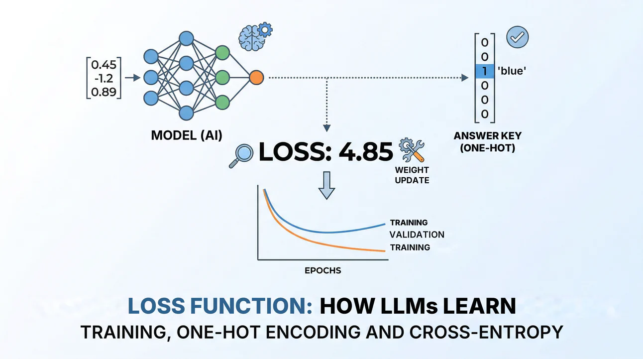
The one and only goal of a neural network
Put very simply, the loss function is a mathematical formula that acts like the big SAT grader for an AI. It evaluates the result the model generated, compares it with the real answer key and spits out a number saying how wrong the neural network is. During the training phase, the model’s one and only purpose in life is to try to push that number down as far as possible.
But to understand how it does that, we need to look inside a neural network. Think of the network (an LLM like GPT, Gemini or Claude, for example) as a gigantic graph, made of nodes (the neurons) and edges (the connections). The magic happens in how the network’s famous parameters (which split into weights and biases ) are distributed in there.
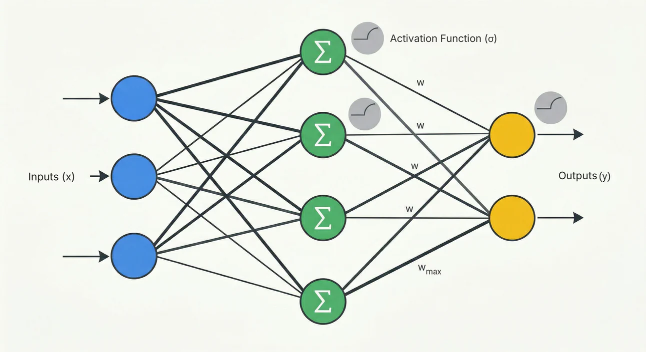
And of course, the input data travels along the edges. But before moving on, what exactly is this “input data”? A neural network can’t read text in Portuguese or English. Remember the Logits article: if you write the word “sky”, the model first turns that token into a long list of numbers (a mathematical vector called an Embedding). So when we talk about “input data”, picture a vector of decimal numbers (like [0.45, -1.2, 0.89, …]) coming in through the front door of the network’s first layer. Those numbers are what travel along the edges.
And each edge carries a multiplier called a weight. When the input data passes through there, it gets multiplied by that weight. When the AI is learning and correcting its mistakes, it’s exactly the weights of those edges, those multipliers, that get changed. The nodes (neurons), on the other hand, are the processing hubs: they receive all the multiplied values coming from the edges, add everything up, add a constant (the bias) and, finally, apply a mathematical formula (the Activation Function). The result of that formula at the node is what generates the new value to be fired off to the next layer of the network.
At the beginning of training, those billions of values are set completely at random. It’s like a student taking an exam where he guesses every answer without even reading the questions. Obviously, the Loss Function takes that random answer, compares it with the perfect answer key and gives the network a mathematical “telling-off”, resulting in a sky-high Loss.
And here comes the heavy engineering. The model doesn’t “think” about writing pretty texts. Its one existential motivation is to minimize that error number, that Loss. To lower the Loss on the next guess, the network needs to figure out which of those billions of weights contributed to the error and in which direction to adjust them to try to get better answers according to the training answer key.
In deep models (Deep Learning) with hundreds of layers, this process is gigantic. The Loss at the very end has to reach all the way back to the first layer of the network. Training an AI model is basically an endless repetition of this cycle of “guess, calculate the Loss, propagate the error back and adjust the weights”, turning random guesses into well-trained neural networks.
The Answer Key and “One-Hot Encoding”
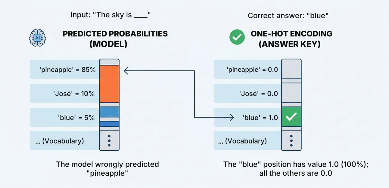
Going back to the example I gave in the Logits article, trying to complete the sentence: “The sky is ____”. Imagine we’re training an LLM from scratch. As we saw before, the model processes the text and the last layer spits out the logits, which after the Softmax function become probabilities from 0 to 100%. Suppose our answer key for completing this sentence is the token “blue”, but since our model was just born and its weights are still random, it generated the following probabilities for the next token:
"The sky is ____"
- “pineapple” = 85%
- “José” = 10%
- “blue” = 5%
- …
Following those probabilities, the answer it gave was: “The sky is pineapple”. Got it wrong, and badly. But how do we translate this “answer key” into math? We use a technique called One-Hot Encoding. Basically, we create a vector of the exact same size as the vocabulary (e.g., 100,000 words/tokens), where the position of the correct word (“blue”) gets the value 1.0 (100%) and absolutely all the others get 0.0. That’s the ideal world the AI needs to try to imitate.
The Math of Cross-Entropy
This is exactly where the Loss Function comes in. For language models, the industry-standard loss function is the Cross-Entropy Loss, but there are many other loss functions out there.
Just out of curiosity: “Entropy” is a concept from Information Theory that measures the uncertainty or the surprise of an event, and “Cross” means we’re measuring the difference (crossing) between two probability distributions: the model’s and the real world’s (the answer key). That’s why this loss function has that name.
The math behind it takes the probability distribution the model made up and compares it with the answer key in the form of a “1” and lots of “0"s from the One-Hot vector. Let’s take a look at its mathematical formula. Don’t panic:
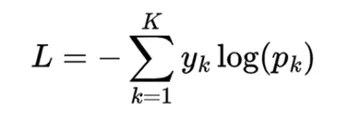
Where:
- K is the size of our vocabulary (e.g., 100,000 tokens)
- y(k) is the real value from the answer key (which is 1 for the right word and 0 for everything else, thanks to One-Hot Encoding)
- p(k) is the probability (between 0 and 1) the model predicted for that token
The big trick of this formula is the summation (∑). Since our answer key y(k) is equal to zero for 99,999 words in the vocabulary, anything multiplied by zero is zero. The whole calculation “collapses” and ignores all the wrong words. The formula only focuses on the probability the model gave to the right word. Mathematically, this is done using the logarithm, and its behavior here is perfect for punishing the AI. It works like this:
- If the model is very sure and predicted 0.99 (99%) for the correct word, the logarithm of 0.99 is a number very close to zero. The Loss ends up super low. The model got it right and doesn’t need to be corrected.
- But if the model got it badly wrong and predicted a probability of only 0.05 (5%) for the right word, the logarithm of 0.05 is a giant negative number.
And that’s why there’s that minus sign (−) in front of the whole formula. It takes that huge negative number and flips the result into a huge positive number. The result of this calculation is a scalar value (let’s say, a nice 4.85, which is huge for this magnitude). That’s the final value of our Loss: a gigantic mathematical “telling-off” saying the AI needs to adjust its weights urgently, because it gave a minuscule probability to the correct answer.
Batches and Backpropagation
In practice, the AI doesn’t calculate the Loss for one sentence and update everything right away. That would be too slow and unstable. It processes a Batch with thousands of sentences at the same time, and the final Loss is the average error across all those examples.
With that average number in hand (our 4.85), an optimizer algorithm (usually AdamW) uses a brilliant technique called Backpropagation to calculate the Gradient Descent (which I’ll explain better in another article). It goes back from end to start through the whole neural network, figuring out how much each of the billions of parameters contributed to that error. Then, it adjusts those weights just a tiny bit (using the “Learning Rate” to define how much that “tiny bit” is), in the exact direction that would make this Loss go down next time.
The AI repeats this process of guessing, getting it wrong, calculating the batch loss and adjusting the weights billions of times, until it stops predicting “pineapple” and starts giving 99% chance to the token “blue”, the right answer.
What the developer actually sees
Day to day, people who train AI don’t sit there staring at loose numbers in the terminal. We keep track of the exact Loss value (ideally it keeps going down with every round of training), and a curve of how it’s evolving over the neural network’s training steps.
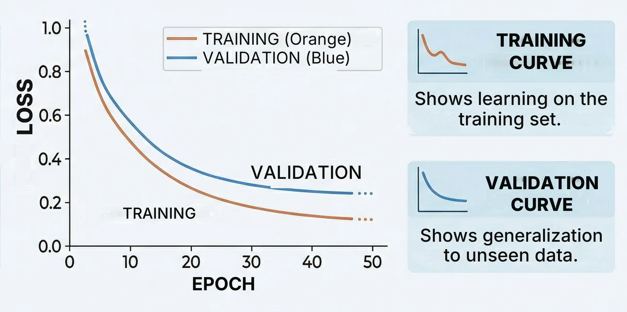
And the idea is to monitor two main lines: the Training Loss (the error on the data the AI is studying) and the Validation Loss (the error on a surprise exam with data it has never seen). If the Training Loss keeps falling, but the Validation Loss starts to rise, the alarm goes off: we have Overfitting, meaning the AI stopped understanding language and started just “memorizing” the training set. That means it probably won’t do well on other surprise exams from the real world. In AI lingo, we say this is a model that “generalizes” poorly.
Getting Your Hands on the Code (PyTorch)
If you want to play with code in PyTorch, you can see the implementation of this:
import torch
import torch.nn as nn

# Let's simulate a vocabulary of 4 words: [blue, beautiful, pineapple, Maria]
# The model processed the sentence and generated these raw LOGITS (no Softmax yet)
# Notice that index 2 ('pineapple') got the highest logit (5.3)
logits = torch.tensor([[-1.2, 0.5, 5.3, -0.1]])

# Our answer key (target) is index 0 ('blue') - PyTorch does the One-Hot internally!
target = torch.tensor([0])

# Instantiating the loss function
loss_fn = nn.CrossEntropyLoss()

# Calculating the error!
loss = loss_fn(logits, target)

print(f"Loss value: {loss.item():.4f}")
A super cool software engineering detail here: in practice, PyTorch’s nn.CrossEntropyLoss() method already applies the Softmax together with the logarithm calculation under the hood. Doing both mathematical operations together is much faster and numerically more stable than doing the Softmax first and calculating the loss afterwards! That’s why we pass the raw logits straight into the function.
And that’s more or less it! :) Understanding how Logits connect with the Loss Function and how it guides the gradients is understanding the real learning engine of any modern AI model. Knowing how the sausage is made changes the game.
Happy studying!