[TUTORIAL] How to fine-tune and teach a new language to a voice model (TTS)
Published on
How long do you think it takes to teach a new language to an artificial voice? In my case, 1 hour of GPU training (it was 15 minutes on 4 H100s, which comes to 1 hour on a single GPU) to teach Catalan to an open voice model that didn’t know a single word of it. The rest of the project was deciding what to teach and listening to LOTS of generated sentences.
The result is called vermut-tts. Vermut is the most popular Catalan aperitif for the weekend, with a packed bar and friends chatting. And that was the target: a model focused on conversational Catalan, nothing like an audiobook narrator.
Oh, and the model is already available on Hugging Face! To use it, just send it any text and it generates the audio for you, and you can even use your own voice.
This is a tutorial with the whole path, in the order I trained things. It works as a map for anyone who wants to teach another language to a similar voice model (the recipe was only tested on Catalan, but it was written so it can carry over to other languages). Throughout the text I explain the general idea of each step and then show what vermut-tts did with it.
Ready? Let’s go!
Listen to what vermut-tts can do:
Laughter in the middle (female voice)
«Em vaig quedar adormida a l’autobús, [laughter] imagina’t.» “I fell asleep on the bus, [laughter] just imagine.”
Laughter at the end (male voice)
«Vinga, va, que t’ho dic de debò. [laughter]» “Come on, I’m telling you for real. [laughter]”
Before you start: what you need in your backpack
Two ways to read this
Just want to understand (or explain it to someone)? Read the text, look at the figures and skip the code boxes.
Want to build your own? Then you’ll need Python, a GPU (graphics card) rented for a few hours and the code that shows up along the way (the environment to run everything is right below). A heads-up: what this text gives you is the map (what to train, with what kind of data, how to check each step), the code for the checks and the cuts, and the numbers for what worked. The training command is left out (its starting point is the recipe that CosyVoice 3 itself publishes).
And for those who want to replicate it, there’s a checklist that’s better to go through now. Finding out you’re missing one of these things halfway through hurts (and costs GPU hours). The two items marked (flexible) can be worked around in part, but for the others there’s no shortcut.
- A listener with a good ear for the language (a native, preferably): willing to listen and give feedback LOTS of times. It’s the most irreplaceable item of all.
- Transcribed audio in the target language (flexible): in this example I used about 65 h of long-form speech (about 90% speeches, the rest reading and news) and about 8 h of real conversation. That’s just so you have an idea of the order of magnitude. I never tested with less, but in my case, hours of good, well-cut audio were worth far more than having many more hours.
- Data-center GPUs for a few hours: about 3 hours of H100 for the whole recipe, adding everything up (Stage 1 alone is 1 hour on one GPU, or 15 minutes on 4). Hourly rental does the job.
- Knowing Python and the command line: at a modest level: installing, editing a configuration, running. An LLM can help you with that.
- A base model with a public speech tokenizer: the “annotator” (the first thing to check in the Preliminary test).
- A base that publishes its training recipe (flexible): that’s what you start from to teach a new language (CosyVoice 3 publishes its own). Even better if someone has already taught a new language to this family of models.
Setting up the environment
If you’re going to follow the steps and code along, read this section. If not, you can skip to the next one.
The base model is about 10 GB, and the alignment script downloads the aligner by itself the first time (torchaudio’s MMS_FA: a few more GB, and a CC BY-NC 4.0 license, for non-commercial use only). The ASR transcriber (automatic speech recognition: it listens to the audio and writes down what it understood) is up to you: any one that covers your language will do. If you can, use one to separate the good takes from the bad ones and another one, which didn’t help choose anything, to give the score.
setup.sh · runs on its own (downloads about 10 GB)
# 1. CosyVoice's code, pinned to a commit
git clone --recursive https://github.com/QwenAudio/CosyVoice external/CosyVoice
git -C external/CosyVoice checkout 074ca6dc9e80a2f424f1f74b48bdd7d3fea531cc
git -C external/CosyVoice submodule update --init --recursive
pip install -r external/CosyVoice/requirements.txt
pip install librosa soundfile jiwer          # jiwer is what computes the CER
# (its list of libraries is not the environment I tested)

# 2. the base model, Fun-CosyVoice3, which doesn't know Catalan yet (about 10 GB)
MODEL=FunAudioLLM/Fun-CosyVoice3-0.5B-2512
MDIR=external/CosyVoice/pretrained_models/Fun-CosyVoice3-0.5B
python -c "from huggingface_hub import snapshot_download; snapshot_download('$MODEL', local_dir='$MDIR')"
Ran without errors? Then the environment is ready.
How a TTS (text-to-speech) model speaks
Before training anything, let’s understand how a machine speaks. The system I used is from the codec-LM family (a codec turns sound into symbols and back, and the LM is the language model that writes those symbols), and honestly the idea is simple. Generating speech becomes the same problem as predicting the next word/token to complete a sentence, like ChatGPT or your phone’s autocomplete, except that here the word/token is a tiny piece of sound, smaller than a phoneme.
In this family of CosyVoice models, imagine an alphabet of 6,561 letters, each one a little piece of sound lasting 40 milliseconds. Since 40 milliseconds × 25 = 1 second of speech, every second becomes 25 “sound letters” from this alphabet. In more technical terms, each letter is a token (or “symbol,” as I’ll call them in this tutorial to make it easier to follow).
Who writes in this alphabet? A dubbing studio with four employees, each in charge of a single thing:
- The actor (the language model, the LM) reads the script and decides how to pronounce that text: which sounds, what rhythm, where to pause. Along with the script comes a director’s note, the instruction, which in vermut-tts is a sentence in Catalan: «Parla en registre col·loquial, ritme normal, en català central.» (“Speak in a colloquial register, normal pace, in Central Catalan”). The actor “speaks” in symbols.
- The annotator (the speech tokenizer) does the opposite of the actor: it listens to any recording and writes down what it heard in those same symbols. It only annotates.
- The mixing desk (the flow matching decoder) turns the symbols spoken by the actor into a “picture of the sound” (the sound drawn out, also called a mel spectrogram, which shows time horizontally, low and high pitch vertically, and volume as brightness), already with the timbre of a specific person.
- The loudspeaker (the vocoder) turns that picture of the sound into real sound, to be played, at 24,000 measurements per second.
Of course, these are analogies: when you open the code, these characters will have other names:
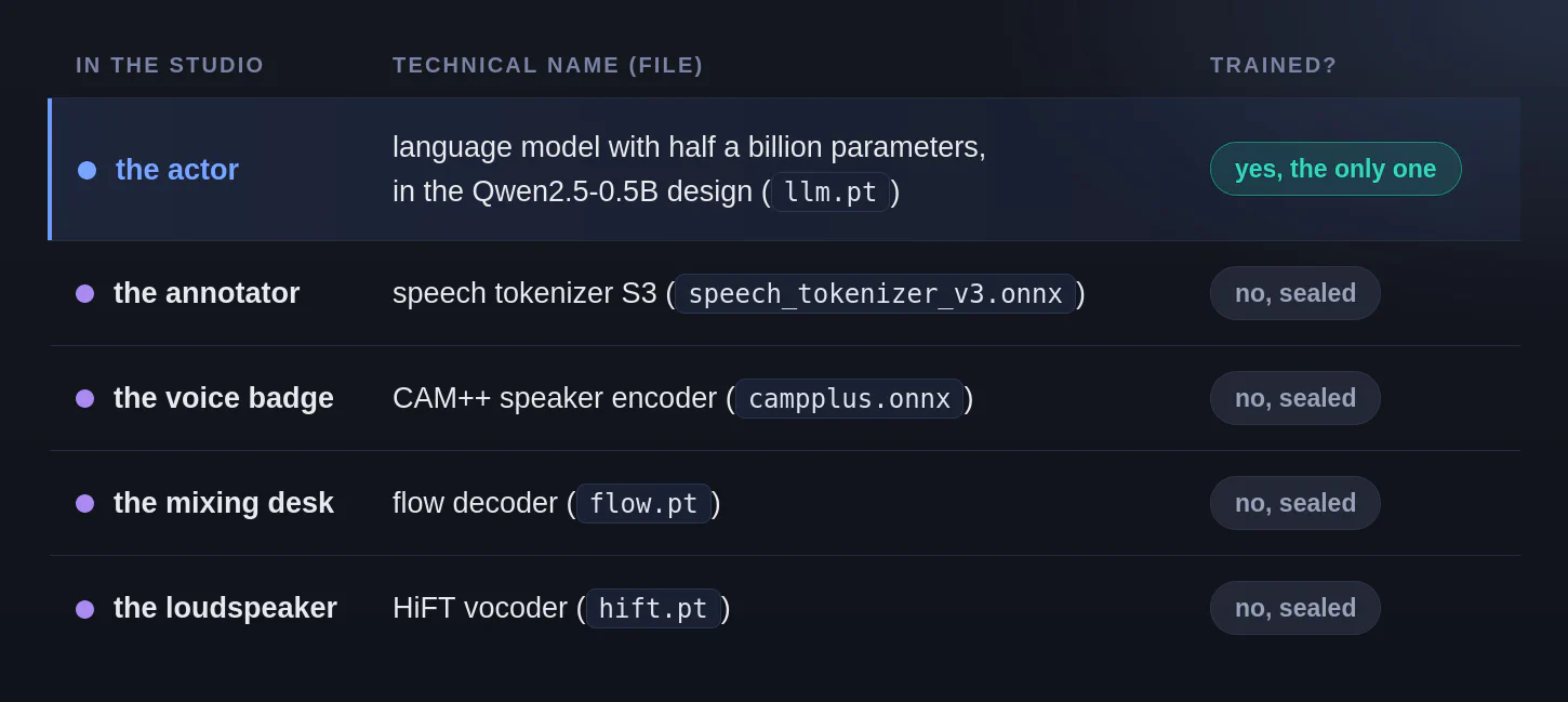
But we had said four employees, so why are there five networks? The fifth isn’t exactly an employee, it’s just the voice badge (the speaker embedding, in the jargon, computed by the CAM++ speaker encoder). In practice, it’s the voice that will be used to pronounce those sounds. The voice badge is 192 numbers that say who is speaking, taken from a reference recording.
The strategy fits in one sentence: I rented the whole studio ready-made and trained only the actor (the language model, the llm.pt). The studio is Fun-CosyVoice3-0.5B-2512, an open model (Apache-2.0) that speaks nine languages (Chinese, English, Japanese, Korean, German, Spanish, French, Italian and Russian), but not Catalan.
The original model learned from about 1 million hours of speech (which is A LOT, impossible to replicate at our level). But to do this initial fine-tuning for a specific language, I used about 65 hours. To compare orders of magnitude, if that 1 million hours were a soccer field, my 65 hours would be the size of a bar table (maybe the very table where Catalans drink their vermut). That’s why the training process doesn’t take that long. Training works like this:
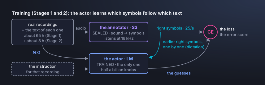
Notice that training has two tracks. On the top one, a real recording in Catalan goes through the annotator, which writes down its correct symbols (25 per second) and serves as the answer key. On the bottom one, the text of that same recording (together with the instruction, the director’s note) goes into the actor, and its job is to guess those same symbols. The light-blue arrow going down to the actor is the dictation (teacher forcing, in the jargon), which works with the actor receiving, at each step, the correct symbols that have already gone by and only trying to guess the next one. In the CE circle (for cross-entropy, a very common language-model loss, nothing exotic), the actor’s guesses are compared with the answer key and turn into the loss, the error score (the lower, the better). Training turns the actor’s half a billion knobs (its parameters) to lower that score, and touches only those.
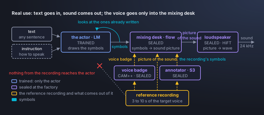
When it’s time to actually use it, the actor receives only the text and the instruction (the way of speaking) and predicts the symbols one by one, looking at the ones it has already written itself (the light-blue loop). The mixing desk turns that line of symbols into a picture of the sound, and the loudspeaker turns the picture into real sound.
And the voice? Remember that the symbols hold, in little pieces, what is being said (and, in large part, how). The reference recording (it’s where the voice badge comes from), which only the mixing desk hears, decides who is speaking. In the instruction format I trained, the actor never receives the recording and, because of that, switching voices costs zero training.
To get a feel for the scale of the symbols, let’s do a calculation.
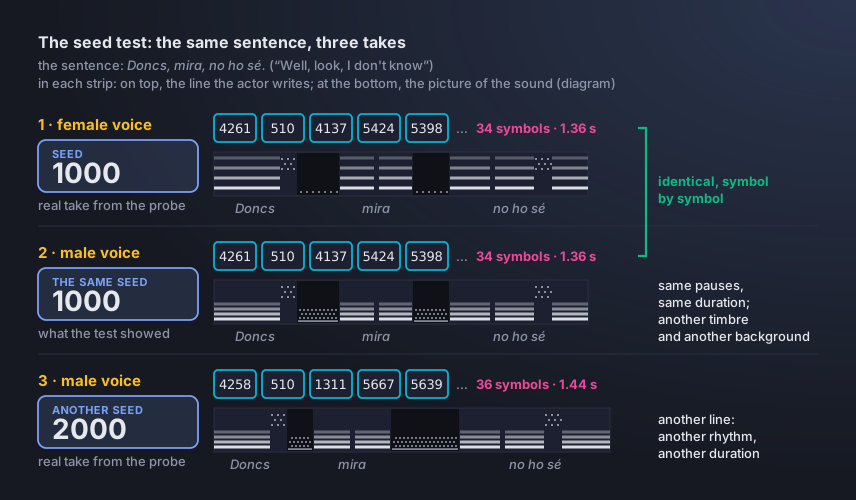
The sentence «Doncs, mira, no ho sé.» was requested four times. So that we don’t get four identical audio files, we change the “seed” (a number that fixes the draw of the symbols the actor picks: each seed gives a slightly different version). The calculation is the same for any of them: symbols ÷ 25 = seconds of speech. With the first seed, the actor wrote 34 symbols, and 34 ÷ 25 = 1.36 s; the other three came out at 31, 36 and 35 symbols (1.24 s, 1.44 s and 1.40 s). Each symbol becomes 960 measurements (at 24 kHz). In other words, the actor decides the duration by itself, and each draw gives a different one.
The first take (female voice, version with 34 symbols, 1.36 s), raw, without any finishing:
But there’s a risk in training this way. For example, if the base model’s annotator hadn’t learned some specific sound of the language you want to teach (in my case, Catalan), that sound would vanish forever, and no training of the actor could teach it.
Imagine a foreigner who hasn’t learned a sound of Portuguese yet. They say “áo” (with an open “a”) instead of the nasal “ão”, because they swap the sound they don’t know for the closest one they have. An annotator without that sound would make the same swap, writing down the symbol of the closest sound. To make sure this problem won’t happen in your training, I recommend running a round-trip Preliminary test.
Stage 0: preliminary test and setting up the metrics
This is the section almost nobody wants to read and the one that saves the most money. A gate is a cheap test that is run before the real trainings. A gate that fails in the preliminary test costs hours, and the same discovery three weeks later costs… the three weeks.
The round-trip test
If you’ve ever tried saving a photo of yourself as a tiny JPEG and opening it again, you’ve probably noticed that the quality got worse and, looking at the pixels, you’ll see more blocky squares at the edges, the strands of hair turned into a smudge and there’s no way back to the original with any retouching. Running this round-trip test is something similar, but with sound. We take a real recording of a human and send it to the annotator (the speech tokenizer), which writes that recording down (16,000 measurements per second become 25 symbols, a 640× compression). Then, the desk and the loudspeaker (the flow and the vocoder) rebuild the sound. Finally, you listen to check that all the sounds are right. If the annotator’s alphabet doesn’t have the symbol(s) for some sound of your language, you’ll notice the wrong pronunciation (like “áo” instead of “ão” in Portuguese, if it doesn’t have the nasal sound).
If that happens, no training invents that letter and, since the pieces come sealed, if this test doesn’t pass, you’re better off switching base models.
In technical terms, what we do here is pass a real audio file through the encoding and decoding process, and after that a listener has to confirm that the resulting audio lost nothing. Notice there’s a catch: the target is to sound as natural as the real audio, not just to be “intelligible” (you can be 100% intelligible and sound like a GPS voice, and that’s not what we want).
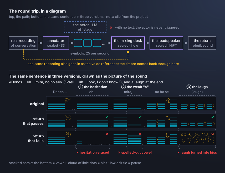
To run this test:
- Grab 2 to 4 real conversation recordings, with hesitation and some laughter (studio reading is the easy case, and doesn’t count).
- In CosyVoice (from the environment you set up at the start), run
inference_vc(clip, clip): the same file goes in as content and as voice, and with no text the actor is never triggered. In another model it’s the same move: pass the audio through the speech tokenizer and the decoder, without the language model in the middle. - A native speaker compares the original and the return, without looking at any number, and decides before running what counts as “passed”. Laughter matters if you want to keep it as a tag in the final model, because an annotator built only on reading may have learned to discard laughter as noise.
In code, the round trip fits in a short file (the first lines just swap torchaudio’s audio loading for soundfile, which doesn’t need torchcodec or ffmpeg).
round_trip.py · needs CosyVoice and a GPU
# round_trip.py: the recording goes through the annotator (tokenizer), the mixing desk (flow) and the loudspeaker (vocoder), without the actor (LM)
import sys
from pathlib import Path

import numpy as np
import soundfile as sf
import torch
import torchaudio

COSY = Path("external/CosyVoice")
sys.path.insert(0, str(COSY))
sys.path.insert(0, str(COSY / "third_party" / "Matcha-TTS"))

# recent torchaudio requires torchcodec+ffmpeg to load audio; soundfile needs neither
def _sf_load(path, *a, **k):
    src = path if hasattr(path, "read") else str(path)
    w, sr = sf.read(src, dtype="float32", always_2d=True)
    return torch.from_numpy(w.T.copy()), sr

def _sf_save(path, tensor, sr, *a, **k):
    sf.write(str(path), np.asarray(tensor.detach().cpu().T, dtype=np.float32), sr)

torchaudio.load = _sf_load
torchaudio.save = _sf_save

from cosyvoice.cli.cosyvoice import AutoModel   # noqa: E402  (only after the sys.path and the patch)

cosy = AutoModel(model_dir=str(COSY / "pretrained_models/Fun-CosyVoice3-0.5B"))
sr = cosy.sample_rate

for clip in sys.argv[1:]:                       # python round_trip.py chat1.wav chat2.wav
    # the same file goes in as content AND as voice: with no text, the actor (LM) is never triggered
    chunks = [j["tts_speech"] for j in cosy.inference_vc(clip, clip)]
    w = torch.cat(chunks, dim=1)
    torchaudio.save(f"{Path(clip).stem}_back.wav", w, sr)
    print(f"{clip}: {w.shape[1] / sr:.1f} s")
Each file generates a _back.wav next to the original. Listen to both, one after the other, and decide.
A real round trip (an excerpt from a travel-booking call, from a corpus of dialogues)
Original (female voice, real recording)
The return (rebuilt only from the symbols, without the actor)
«L’hora de sortida que li he dit és a les nou però hi ha per exemple un Altaria que surt a les nou i cinc, exactament, aquest li seria just.» “The departure time I gave you, sir, is at nine, but there’s, for example, an Altaria (a Spanish train) that leaves at five past nine, exactly, and that one would be cutting it close.”
Detectors and the blind kit
Another thing worth implementing is an ASR transcriber (a speech recognition model that listens to an audio file and transcribes what it understood). With it, we can get some important metrics, like the CER (character error rate), the percentage of wrong letters. This is also where a classic Data Science concept comes in: comparing precision and recall. Why? It’s how you test a smoke detector: precision measures whether, when the detector went off, there was really smoke; recall measures, out of all the smoke that existed, how much the detector caught.
To see the math in a real case, I’ll use a second instrument, a phoneme recognizer (it writes down the sounds it heard instead of letters; phonemes are the sounds a language uses to tell one word from another, like the /p/ and the /b/ in “pat” and “bat”). I used one to keep track of the Catalan /ʒ/, the “j” of «jo» and «ja», which the model sometimes swapped for the “y” of “yacht”. Here the detector is the recognizer, and the smoke is the /ʒ/ sound. So it “goes off” when it writes /ʒ/ for the stretch it heard. Precision measures whether, when it went off, the /ʒ/ was really there; recall measures, out of all the /ʒ/ that existed, how many it caught. The one who checks whether the /ʒ/ really existed is your ear, listening to the result.
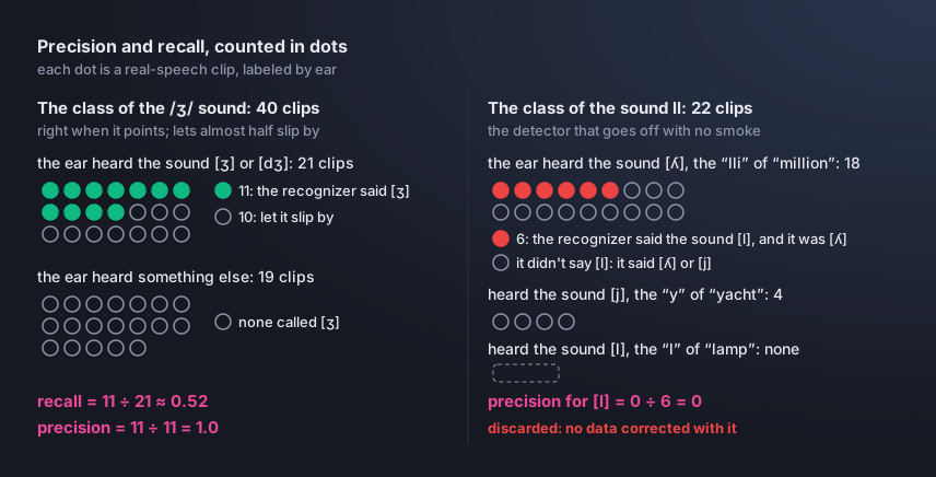
In numbers, precision is flagged correctly ÷ flagged, and recall is flagged correctly ÷ had the sound (in the figure, 11 ÷ 11 and 11 ÷ 21). In other words: when the recognizer goes off, it really is /ʒ/ (precision 1.0), but it lets almost half of the real /ʒ/ slip by (recall 0.52). That’s why its number is good for comparing versions, never for counting hits.
The transcriber is an ASR that covers your language (I used a Whisper large-v3 tuned for Catalan). There’s just one golden rule: ideally, whoever gives the score hasn’t helped choose anything, otherwise it’s a student grading their own exam. That’s why I use two ASR transcribers, one to separate the good takes from the bad ones and another one, which took part in no choice (of model, of pair or of checkpoint, that “video game save” of the model), to give the score.
For the code below, which has the CER, before counting, norm_text() strips tags, punctuation and capital letters (a misplaced comma isn’t a pronunciation error), and jiwer counts the wrong letters.
measure.py · runs on its own (pip install jiwer)
# measure.py: the CER, the percentage of wrong letters
import re
import unicodedata

import jiwer                                   # pip install jiwer

def norm_text(s, keep=""):
    """lowercase, without [..] or <..> tags and without punctuation. keep: the marks that are part of
    your language's spelling (in Catalan, the middle dot of l·l: keep="·")"""
    s = s.lower()
    s = re.sub(r"<[^>]+>|\[[^\]]+\]", " ", s)
    s = "".join(c for c in s if unicodedata.category(c)[0] != "P" or c in keep)
    return re.sub(r"\s+", " ", s).strip()

def cer(text, hyp, keep=""):
    """fraction of wrong letters between the requested text and what the ASR transcriber heard"""
    ref, h = norm_text(text, keep), norm_text(hyp, keep)
    return jiwer.cer(ref, h) if ref else float("nan")          # 0.042 = 4.2%

if __name__ == "__main__":
    # punctuation and capitals don't count; the "é" that became "e" does: 1 wrong letter out of 19
    print(cer("Doncs, mira, no ho sé.", "doncs mira no ho se"))     # 0.0526
I also used a laughter detector (the jrgillick/laughter-detection), which was trained on English audio, so I first checked on the corpus of real Catalan recordings whether it worked there too. Out of 40 sentences with the [laughter] tag, it found the laughter in 88% (recall 0.88), and out of the 60 without the tag, it went off by mistake in only 2.
But of course, it only answers “was there a laugh?”. To know whether the laugh sounded natural, that will depend on your ear too.
Two instruments and one rule are still missing:
The probe is the speech therapist’s list (in the jargon, a fixed evaluation set). You know how they ask a child to always repeat the same words, each with a hard sound (“squirrel”, “strengths”), to see where they stumble? It’s that, except the one repeating is the model (in my case, about 270 items among sentences, single words, short expressions and the cases I wanted to keep an eye on, like laughter, grouped by the hard sounds of Catalan).
Each item comes out a few times per version of the model (I used 2 voices × 2 takes, so over a thousand takes), and the ones grading are programs, with the metrics I just explained (the CER, the /ʒ/ detector, the laughter detector, and whatever else you want to measure). Since the list never changes, you can compare one version with another, and nobody has to listen to over a thousand takes. That’s why this probe works as an initial sieve to discard the disastrous audio (swapped word, cut-off ending, hallucination, etc.). What it can’t do is tell, between two good models, which one sounds more natural to the human ear. These metrics are for counting wrong letters and missing laughter, not for naturalness. That’s why I had a “blind kit”, to be judged by a human ear after each training run.
The blind kit is a blind A/B test, meaning the same sentence, in the same voice, pronounced by two different versions of the model, with the sides drawn at random. Then a person votes on which of them came out better (option A or B), whether they came out “equal” or whether both were bad.
For the blind kit, I recommend setting aside unseen sentences just for it, which won’t be used anywhere else in the training.
Stage 1: teaching the new language
Tests passed, time to train. Fine-tuning a model is like teaching Indian cooking to someone who’s already a chef in Italian food. The person doesn’t relearn how to hold the knife, they only learn which ingredients go together in this new cuisine. The base model already knows how to speak other languages; what it’s missing is the connection between written Catalan and the sounds of spoken Catalan. For example, in Catalan, “ll” sounds like the “lli” in “million” (the word «lloc», meaning “place”, is pronounced something like “lyok”). Just from reading the letters, a model that has never heard Catalan has no way of knowing that.
The data I used for this first phase was about 65 hours of recorded and transcribed Catalan. Almost all of it (about 90%) was long-form speech from public speeches in the Catalan parliament, and the rest was reading by professional speakers and news. I told you at the beginning that I didn’t want a model that used the tone of voice of a TV news anchor or an audiobook narrator, but those were the largest collections of transcribed Catalan I could find. That’s why I left the conversational part for Stage 2.
For this stage, I focused on teaching a new language, Catalan. So the most important thing is to use a well-recorded audio corpus, with a good microphone, and a word-for-word transcript. A good transcript includes punctuation, which the actor (the LM) reads as a signal instead of ignoring it as noise (that is, if the sentences come without a period, it raises its pitch on the last syllable instead of lowering it, as it would at the end of a sentence). If your transcripts aren’t punctuated, it’s worth running them through an LLM or running the original audio through an ASR model that already transcribes with punctuation in the right places.
Data: the edges, where each recording starts and ends
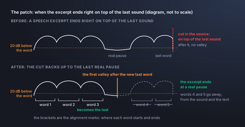
You know that phone video that cuts off while the person is still finishing the sentence? Every training recording has two edges, the one at the start and the one at the end of the speech, and our “actor” will learn how to start and end sentences based on the edges you show it in training. In other words, if every example ends with the last word half cut off, it will learn that sentences end like that and copy that behavior. Unfortunately, that was the case with my corpus of speech data, whose original cut usually landed right on top of the last sound (I listened to 24 excerpts and marked “the ending is missing” in 22 of them, almost all).
To fix this, I ran a forced alignment, which is like a child reading with a finger under each word, only with audio. It marks where each word starts and ends. Then all you have to do is run a pair of scissors through the valley, the first quiet point after the last word (at least 20 dB below it, for 40 to 50 ms), with a short fade (the smooth drop in volume) and without adding anything.
An important detail is that cutting only “where the sound gets quiet” doesn’t work well. Final consonants (like the “s” in “três”) are weak, and a volume-based cut would think it’s silence and chop them off. That’s why the alignment comes first: it says where the last word ends, and the search for the valley only starts after that point, so that final “s” isn’t removed.
Another precaution worth taking is for your scissors not to cut too close to the last word (in one of my collections, more than a third of the excerpts didn’t even have a pause to back up to, which turned out badly, so I threw that data away).
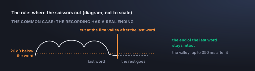
In code, the path has three steps, and the first two get a block. The first aligns: it returns, for each word, where it starts and ends (in seconds) and a confidence score from 0 to 1. The numbers in the text need to be spelled out, because the aligner only understands letters.
align.py · needs torchaudio (and downloads the aligner)
# align.py: where each word starts and ends in the sound (forced alignment with MMS_FA)
import re
import unicodedata

import numpy as np
import torch
import torchaudio

SR = 16000
dev = "cuda" if torch.cuda.is_available() else "cpu"
bundle = torchaudio.pipelines.MMS_FA                 # the first time, it downloads the aligner's weights
fa = bundle.get_model().to(dev).eval()
tok = bundle.get_tokenizer()
aligner = bundle.get_aligner()

def strip_tags(text):
    return re.sub(r"<[^>]+>|\[[^\]]+\]", " ", text)

def words_of(text, keep="'·-"):
    """the words of the text; keep: what can appear INSIDE a word (in Catalan: l·l, d'aigua)"""
    return [w for w in re.split(r"\s+", re.sub(r"[^\w\s" + re.escape(keep) + "]", " ", strip_tags(text))) if w]

def romanise(word):
    """plain a-z, which is what the aligner knows (strips accents, cedillas and marks).
    For a non-Latin alphabet, this is where a romanizer goes (like uroman)"""
    chars = []
    for c in unicodedata.normalize("NFD", word.lower()):
        if unicodedata.category(c) == "Mn":
            continue
        if "a" <= c <= "z":
            chars.append(c)
    return "".join(chars)

def align(x16, text):
    """x16: mono sound at 16 kHz (float32). Returns [[word, start, end, score], ...] in seconds.
    Numbers and acronyms must be spelled out: the aligner only understands letters."""
    words = words_of(text)
    roms = [romanise(w) for w in words]
    keep = [j for j, rm in enumerate(roms) if rm]
    if not keep:
        return []
    with torch.inference_mode():
        em, _ = fa(torch.tensor(x16).unsqueeze(0).to(dev))
    spans = aligner(em[0], tok([roms[j] for j in keep]))
    ratio = len(x16) / em.shape[1]
    return [[words[j], round(sp[0].start * ratio / SR, 3), round(sp[-1].end * ratio / SR, 3),
             round(float(np.mean([t.score for t in sp])), 3)] for j, sp in zip(keep, spans)]

if __name__ == "__main__":
    import sys

    import librosa
    import soundfile as sf

    # python align.py excerpt.wav "the text of the excerpt"
    x, sr = sf.read(sys.argv[1], dtype="float32")
    x = x.mean(1) if x.ndim > 1 else x
    x16 = librosa.resample(x, orig_sr=sr, target_sr=SR) if sr != SR else x
    for word, start, end, score in align(x16, sys.argv[2]):
        print(f"{start:6.2f} {end:6.2f}  score {score:.2f}  {word}")
The second is the scissors: it looks for the first valley after the aligned end of the last word (the criterion is above); with no valley, it tries the quietest point and, as a last resort, cuts 120 ms after the word. The block only covers the end (the start is the mirror image).
cut_at_valley.py · just the functions, no example at the end (needs numpy)
# cut_at_valley.py: the scissors go through the valley (the first quiet stretch after the last word)
import numpy as np

SR = 16000
HOP = 0.01                                      # the volume is measured every 10 ms

def frame_db(w, hop=HOP):
    """the volume of each 10 ms window, in dB"""
    n = int(hop * SR)
    if len(w) < n:
        return np.array([20 * np.log10(np.sqrt((w ** 2).mean()) + 1e-9) if len(w) else -120.0])
    nf = len(w) // n
    return 20 * np.log10(np.sqrt((w[: nf * n].reshape(nf, n) ** 2).mean(1)) + 1e-9)

def _level(db, s, e):
    """the volume of a word that goes from s to e (seconds): the 80th percentile of its windows"""
    a, b = max(0, int(s / HOP)), min(len(db), int(e / HOP) + 1)
    return float(np.percentile(db[a:b], 80)) if b > a else float(db[max(0, a - 5): a + 1].max())

def valley_after(w, db, t_end, wlvl, search=0.35, drop=20.0, hold=0.04, fallback=0.12,
                 min_tail=0.04):
    """Where to cut after the aligned end of the last word (t_end, in s).
    Returns (cut in s, how it was found)."""
    n = len(db)
    T = len(w) / SR
    i0 = int(t_end / HOP)
    lim = min(n, int((t_end + search) / HOP))       # searches up to 350 ms after the word
    k = int(round(hold / HOP))                      # consecutive quiet windows that make a valley
    run = 0
    for i in range(i0, lim):
        run = run + 1 if db[i] < wlvl - drop else 0         # 20 dB below the word
        if run >= k:
            return min(max((i - k + 1) * HOP + hold, t_end + min_tail), T), "valley"
    win = db[i0:lim]
    if len(win) >= 3 and wlvl - win.min() >= 12:        # no valley: the quietest point (-12 dB)
        return min(max((i0 + int(np.argmin(win))) * HOP + 0.02, t_end + min_tail), T), "min"
    return min(t_end + fallback, T), "fallback"         # not even that: 120 ms after the word

def cut_with_fades(w, ta, tb, fin=0.02, fout=0.03):
    """cuts from ta to tb (s) with a cosine fade at each end; adds nothing"""
    a, b = max(0, int(ta * SR)), min(len(w), int(tb * SR))
    y = w[a:b].copy()
    fi, fo = min(int(fin * SR), len(y) // 2), min(int(fout * SR), len(y) // 2)
    if fi:
        y[:fi] *= (0.5 * (1 - np.cos(np.pi * np.arange(fi) / fi))).astype(np.float32)
    if fo:
        y[-fo:] *= (0.5 * (1 + np.cos(np.pi * np.arange(fo) / fo))).astype(np.float32)
    return y

def cut_the_end(w, spans):
    """Where to cut the end of the excerpt. spans: [[word, start, end, score], ...] (from align.py).
    Returns (cut in s, "valley" | "min" | "fallback")."""
    db = frame_db(w)
    last = spans[-1]
    return valley_after(w, db, last[2], _level(db, last[1], last[2]), hold=0.05)
One case the scissors may need to handle is the one I mentioned of excerpts that end right on top of the last sound, with no space after it (mine had them, as Figure 4b shows). If there’s no valley afterward to cut at, what the code does is back up to the last real pause (about 50 ms after the pause starts), and the words that come after that are left out of that audio. If fewer than 3 words or less than 1 second of speech remain, I removed the line (except for single words, which are important). It’s a patch, of course, and it’s only worth writing if your corpus has this defect (that part isn’t in the block).
The third is the final check, and it doesn’t need a block. I ran an ASR transcriber to check each cut piece of audio against the transcribed text, and anything above 35% wrong letters got dropped. In these alignments alone, I discarded about 40% of my corpus (I had over 110 hours before the cut, and ended up with about 65). Text with fewer than 4 words passes straight through, because it can’t be checked, and an empty transcript, in my case, passes too (if you’d rather drop the line in that case, just add that check).
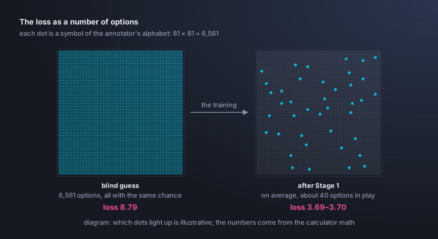
With all of this, the result was that the validation loss (the training error score on an exam of unseen sentences; the lower, the better) practically didn’t change: it went from 3.69 to 3.70. One way to read that number: e raised to the loss is how many options the actor is still unsure about at each symbol. Blind guessing would be 6,561 (loss 8.79); after Stage 1, about 40, as Figure 5 shows.
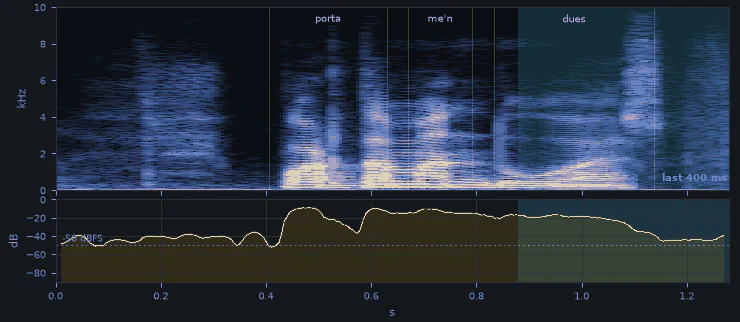
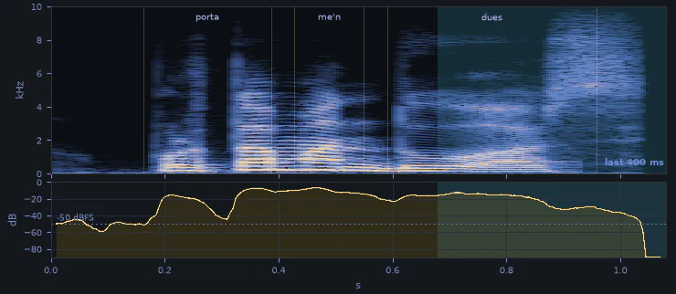
But when I went to listen to the results, it was a different story. I compared, blind, the training with the trimmed edges (65 hours) against the one with the edges as they had come (over 110 hours), and I preferred the corpus that had gone through my “precise” scissors, which got rid of most of the recordings with bad edges.
Another thing that showed up a lot was a breath at the end of the audio (normal, we usually breathe before starting the next sentence), which had been learned from the cuts of the original corpus, but dropped to almost zero in this version with well-made cuts.
Same sentence, two trainings. Listen to what changes at the edges:
Put on headphones and listen to the clips below twice: the sentence and the voice are the same, and what changes is at the start and the end of the speech. Under each one comes the spectrogram (the blue band marks the last 400 ms, and the dashed line is −50 dB).
«Porta-me’n dues.» “Bring me two.”
Old edges (over 110 hours)
Trimmed edges (about 65 hours)
Training: dictation versus essay (the most important difference in this tutorial)
But why didn’t the score change? Because, in training, what the model does is something like a dictation with the teacher whispering the answers (the technical name is teacher forcing):
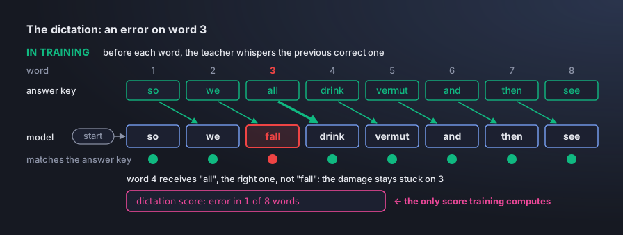
For example, in the drawing above, the sentence is “so we all drink vermut and then see”, and the student gets the third word wrong and writes “fall”. Before generating the fourth (which would carry the previous error and could snowball into an avalanche of mistakes), the teacher whispers the correct word (“all”), and the student carries on from the right place.
When it’s time to really speak, though, it’s like an essay:
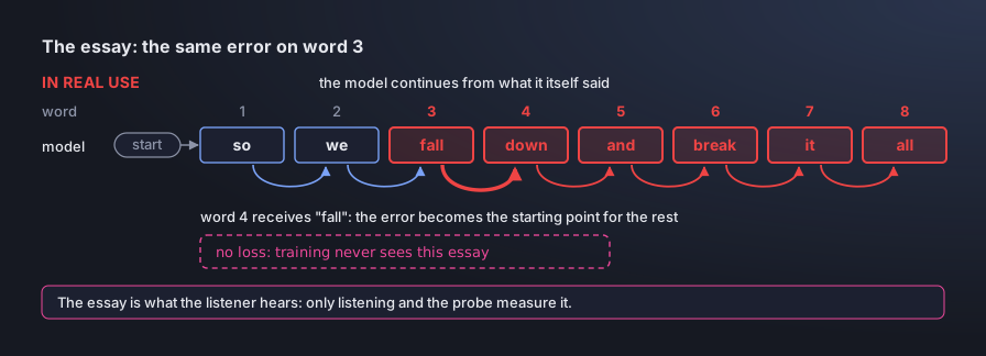
After “fall”, nobody corrects anything, and the sentence can turn into “so we fall down and break it all”. This chain-reaction fall, which the dictation hides and the essay reveals, is what the literature calls exposure bias.
Hence the two-key rule. The validation loss tells you whether training is healthy and when to stop (it levels off at around two epochs, two passes through the data, and after that it’s rote memorization). To approve a new training run, though, you need to listen with a human ear, because the loss only sees the dictation, and the fall only shows up in the essay. Grab about 10 sentences the model has never seen, give each one to it in the training format, let it speak with nobody whispering, and listen to check whether you can understand each one. In vermut-tts, no checkpoint was approved by the loss alone.
In code, the dictation fits in three lines (pseudocode, not the training script):
train_step.py · pseudocode, not the real script
def train_step(text, instruct, real_audio_16k):               # Stages 1 and 2: the recipe trains THIS
    targets = s3_tokenizer(real_audio_16k)                    # the annotator, sealed: sound -> right symbols, 25 per second
    logits  = lm(SOS + bpe(instruct + text) + TASK + targets) # the actor, trained: guess of the next symbol
    return cross_entropy(logits, targets)                     # an ordinary LM loss; nothing exotic
Training: the recipe, item by item
Before listing the recipe, let’s understand where all of this fits. The path of each training line is: the audio and the text come in, the text gets punctuation, the alignment marks the start and end words, the scissors cut the end the right way and the ASR transcriber checks the trimmed excerpt. What’s left becomes a line in a data folder in CosyVoice’s format: wav.scp (where each audio file is), text, utt2spk (who is speaking) and each line’s instruction.
To make it less abstract, here’s one utterance turning into a training line. Each file in the folder keeps one line per utterance, always starting with its id (the id, the path and the speaker are made up; the note is the standard one, the same one the model receives at use time):
data/train/ · the four files, with the utterance id in common
# wav.scp
ex0001 /data/wavs/ex0001.wav

# text
ex0001 Doncs, mira, no ho sé.

# utt2spk
ex0001 spk0042

# instruct
ex0001 Parla en registre col·loquial, ritme normal, en català central.<|endofprompt|>
The file that matters most there is instruct, because it says how that utterance was spoken. It’s the director’s note, “Speak in a colloquial register, normal pace, in Central Catalan”, and each piece of it is a field:
- Register (
Parla en registre col·loquial): the type of speech the recording came from. This is the conversational sentence, which only arrives in Stage 2. In Stage 1 it changes with the source:Llegeix en veu altafor reading andParla com en un discurs al parlamentfor the speeches. - Pace (
ritme normal): the speed of speech, measured in syllables per second. The utterances go into a line, from slowest to fastest, and the line is cut into three groups of the same size, which getritme lent,ritme normalandritme ràpid. It’s like splitting a class into short, medium and tall kids: “normal” is the middle third of my data, not a number I picked. - Volume (
veu altaorveu baixa): the same cut into three groups, only for the volume of each utterance against the median of the speaker themselves. Only the two extremes get the phrase, which is why the line above doesn’t have it. - Variety (
en català central): which Catalan that is, because the language has more than one variety (en català valenciàanden català balearare others). The standard note asks for Central. - Closing (
<|endofprompt|>): the mark that tells the actor where the note ends and the text begins.
In about 10% of the lines the note comes neutral, without any band at all. Apart from that, the set of notes is small and fixed. And why already in Stage 1, if conversation only arrives in 2? Because that way the actor trains from the start in the format it will use later (note plus text) and learns to connect the words of the note to the way of speaking.
From there on it’s CosyVoice’s own recipe, the one in the example examples/libritts/cosyvoice3/run.sh in its repository: stage 0 builds those folders (in their example the instruction is one for all the lines, the “You are a helpful assistant.”; in mine, each line has its own, like the one you just saw), stages 1 to 3 extract the embeddings and the symbols and pack everything into parquet, and stage 5 trains. Only, stage 5 of run.sh loops over llm, flow and hifigan, and the script itself warns that, for now, only the llm can be trained. It’s the actor, and it’s the only one I trained.
So, the recipe:
- Learning rate: a peak, with warmup in the first 5% of the steps and a smooth drop to almost zero (in my case, from
1e-4to1e-6) - Batch (the “pile”): dynamic: by the size of the audio files (sound frames per GPU), not by how many there are, with two batches together before turning the knobs (that’s gradient accumulation). In my case, up to 6,000 frames per GPU, about 120 s of sound
- Budget: counted in steps (each step is a handful of examples going in together and one adjustment to the model’s numbers), not in epochs. Do a short run to measure how many steps the training takes per hour of audio, already with the equal-sized slices (the pitfall just below), and multiply by the hours you have: steps per epoch ≈ hours × steps per hour. In my case it came to about 3 per hour (measured on an earlier run where the epoch had also shrunk, so measure yours): about 65 h × 3 comes to about 200 per epoch, about 400 in two, and the training did 396, in 15 minutes on 4 H100s
- When to stop: at the end of the 2nd epoch (one pass through the data, according to the training program), with the loss stable; a checkpoint (the model’s video game save) every quarter of an epoch
Think of the learning rate I mentioned above as the size of the step of someone trying to come down a mountain trail after dark. Short steps seem safe, but they take too long to reach the end of the trail; long steps get there faster, but you risk overshooting or getting hurt.
Out of the box, CosyVoice doesn’t have the smooth learning-rate drop that I used (it’s one of the patches I applied). Either you apply a similar patch, or you use the scheduler it already has and accept that the curve will look different from mine.
A pitfall in CosyVoice’s training program: the one that decides when an “epoch” ends is the code, and it closes the epoch for all GPUs as soon as the first one runs out of data. Imagine a supermarket with four checkouts, one per GPU, and a manager who closes all of them when the first line empties. It makes no sense. The data arrives in slices (the files each GPU reads, the shards), and mine were 18, of uneven sizes, so each epoch read at most about four fifths of the data, and nobody told me. And, if you have fewer slices than “reading helpers” (the data loader’s workers, 4 per GPU), the same slice is read two to four times.
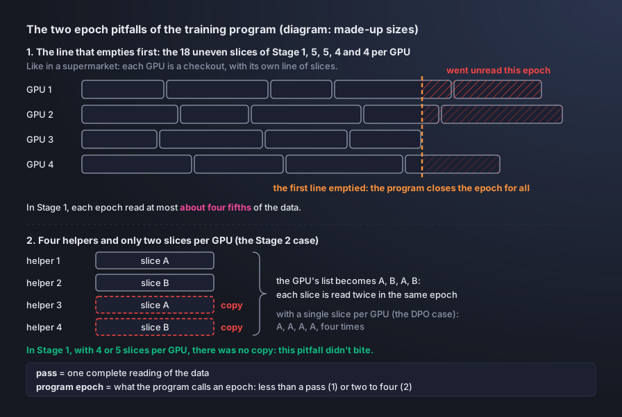
The rule that comes out of this: plan in steps, write the data in equal-sized slices and read each checkpoint’s step counter.
Stage 2: teaching it to converse, with hesitation, laughter and silence
After Stage 1, the model speaks Catalan, only like a TV news anchor or an audiobook narrator, because those were the recordings I gave it. What separates that from a natural conversation between friends is the register (the way of speaking that changes with the situation, from “Dear Sirs” versus “Hey, what’s up?”), but mainly the sound. In natural conversational speech, the pace speeds up in the obvious parts, weak vowels get swallowed, sentences are dropped halfway and restarted, and laughter and breathing are part of the speech.
That’s why Stage 2 is the same recipe as Stage 1, only pointed at real conversation. What I wanted was bar chat, but conversation in that chatty style, and transcribed in Catalan on top of that, is something very rare. In my case it was real dialogues (like customer service calls) from twenty-something people.
I started from the Stage 1 checkpoint and used a learning rate ten times smaller (1e-5), because after the first stage the model already spoke Catalan, and it was just a matter of polishing.
Data: keep and tag, never delete
Ever heard of the concept of disfluency? Those are the quirks we have in natural speech that don’t show up in writing, like the “uh”, the “hmm”, a sentence dropped halfway and restarted, a short laugh, the breathing. In traditional audio engineering that’s garbage to be thrown out, but here, since the focus is a conversational model, it’s exactly the product we want to keep. So the rule becomes: keep the sound and mark in the text what happens there. The “uh” and the “hmm”, instead of being ignored (as they would be in a subtitle), go into the transcript as words; laughter and breathing become specific tags: [laughter] and [breath] (both already exist in CosyVoice’s text vocabulary, but if you’re using a base model without them, you can create them as new tokens). Example:
- Audio (me, in Portuguese):
- “Clean” transcript: “so then we went on Sunday”.
The model concludes that the “uh” and the laughter show up out of nowhere. You taught the model to be random. - Kept and tagged: “so then we, uh, we went [laughter] on Sunday”.
Each sound has a match in the text, and “random” becomes “on demand”.
Data: the model that forgets that sentences can be long
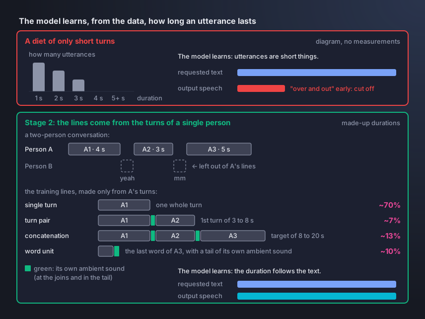
Our real conversations are normally made of short turns (“mm”, “yeah”, “okay”), not super long monologues. In the AI world, the one who decides when speech ends is the model itself, with the EOS symbol, which is the equivalent of the ham radio’s “over and out”. The problem is that if we train the model only on short utterances, it will learn, as a bonus, that utterances are always short things.
To avoid falling into this problem, I tweaked the data. Instead of training only on the turns as they come (short), I put together four types of training line from the same recordings (a training line is an audio file with its transcript). A turn is the stretch in which one person speaks before the other one comes in, and each line uses only the turns of one person (the listener’s “yeah” and “mm” are left out). Figure 8, right below, shows the four types coming out of the same conversation:
- Single turn: one whole turn, the way it came out of the recording.
- Turn pair: two consecutive turns from the same person, joined into a single audio file, with a bit of the recording’s own ambient sound in the middle.
- Concatenation: several consecutive turns, joined the same way, until they add up to about 8 to 20 seconds.
- Word unit: just the last word of a turn, with about 80 ms of the recording’s own ambient sound after it (otherwise the model learns abrupt endings).
The pairs and the concatenations teach that an utterance can be long. The word unit covers the other extreme, a single word on its own (like “yes”, “no”, “already”), which is a hard request for the model. Adding it all up, the lines go from one word to about 20 seconds, and that’s how the model learns that the duration of speech follows the requested text.
Data: silences teach a lot too
Notice that, between two joined turns or at the edge of a recording, something has to fill the silence, that background “ambient sound” of the recording that exists when nobody is speaking (the “room tone”). The temptation is to paste in any ambient sound at all (collected from another moment, generated by a program or an artificial silence of “zeros”). But the actor learns the acoustics of the pauses together with their position.
There’s a metric, the symbol diversity, which is computed by counting how many of the symbols used are different and dividing by the total. With letters it’s easy: “banana” has 6 letters and 3 different ones (b, a, n), so 3 ÷ 6 = 0.5. A sequence of 20 letters “z” has only 1 different letter, so 1 ÷ 20 = 0.05. Close to 1 is varied, close to 0 is repetitive.
A real, clean conversational pause gives about 0.45 (out of every 100 symbols, about 45 different ones), because real ambient sound fluctuates all the time, and so does its annotation. Fake pasted material gives only about 0.10 to 0.19. And the model can learn that poorly made hack. Then, the mixing desk and the loudspeaker (the flow and the vocoder), which just obey, turn that pile of symbols into sound, which can end up sounding like an artificial breath, a hiss or, in the case of zeros, a dead hole. None of those is good for us.
And this really showed up in my data. At first, I tried filling the pauses with ambient sound collected from somewhere else, and a breath detector found breathing in 20 of 20 of those excerpts, because the collected “silence” was, for the most part, people in the recordings breathing between one sentence and the next. In another version where I pasted a synthetic ambient sound (generated noise) at the ends, 18 of 20 training clips sounded like a “hiss at the end”.
Below I show the same sentence read, one with ambient sound and one with only zeros. With headphones, you can hear the gap between «Corfú» and «també». With the ambient sound, there’s still a natural, very faint hiss, but with zeros, the gap is empty and sounds artificial:
With the ambient sound (male voice, original pause)
With zeros (male voice, middle of the pause zeroed out)
«I després la ciutat de Corfú… també és molt interessant.» “And then the city of Corfu… is also very interesting.”
Training: the same recipe, with few changes
The recipe is the one from Stage 1, and what changed fits in a list:
- Starting point: the Stage 1 checkpoint, the one from the second epoch. Only the actor (the
llm) is trained, in the instruction format: the director’s note plus the text, no voice sample. - Learning rate: constant
1e-5, ten times smaller than the Stage 1 peak. - Minimum length: the training program discards lines shorter than a minimum (I used 0.5 s). I lowered it to 0.35 s, otherwise the word units, which are tiny, would be gone.
- Slices: 8, of the same size, 2 per GPU, which gives 72 steps per epoch. It’s the Stage 1 pitfall again: with uneven slices, one of my runs trained only 55, 31 and 33 steps in the three epochs.
- Epochs and checkpoint: 3 epochs, with one checkpoint per epoch. On the probe the three were within the noise, so I took the second one to the blind kit (the way of speaking is invisible to the dictation score), and it beat the previous run. It’s the checkpoint the program calls epoch 1, because it counts from zero.
- Cost: about 20 minutes on 4 H100 GPUs. The expensive part of this stage was building the data editions and listening to the kits.
The model’s voice
Think of a keyboard with a sampler. The musician records one note from a real violin, and from then on the keyboard plays any melody with that timbre, without ever having learned the violin. In the same way, if the recording has a hiss, every melody generated from that sampler will have a hiss. The one playing is the actor, and the sampler is the reference recording.
The program takes from that recording the voice badge, plus its symbols and its picture of the sound (the mel spectrogram), hands everything to the mixing desk (the flow) and forgets it. In other words, there’s no training, and adding a new voice is practically free.
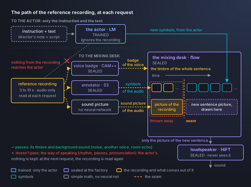
So, to pick a good reference recording for the voice, the ideal is to use about 10 seconds of continuous speech, clean and from a single person, preferably in a conversational style.
The actor picks each symbol based on probabilities, and the seed is the numeric value we set that fixes that choice. With the same seed, the same text and the same instruction, the line of symbols the actor writes should come out exactly the same (on the same equipment). The way of conversing comes from the model’s training, and every voice you bring to be cloned or to serve as a base will speak in the model’s way, not the recorded person’s.
Stage 3: DPO, teaching by preference
After the two stages, the model speaks bar-chat Catalan, but it can still sound odd at times to someone listening closely. In my case, the most visible issue was the laughter tag. In the 28 sentences I generated with the [laughter] tag, the laughter detector found laughter in 19 (68%), but it often came after a weird pause, not very natural.
No machine can automatically measure whether “that laugh sounded like a real person’s laugh?”. But a human listener can. To turn that into training there’s DPO (direct preference optimization), and its idea fits in a singing lesson.
The singing lesson
In Stages 1 and 2, the teacher sings the right note and you imitate it. In DPO, the student sings in two tones and a judge says which one came out better. It’s kind of like an A/B test, where the model generates two or more versions of the same sentence, and a human listens to both and says “the second one was better”.
In my case, I made the model generate the same sentence six times for each voice (male and female), and the takes come out different because I used different seeds to pick the probabilities of the vocabulary’s symbols.
After picking the best ones, I ran one more training, whose idea is to make our actor (the LM) more likely to choose the symbols used in those winning takes, and less likely to choose the symbols used in the losing takes.
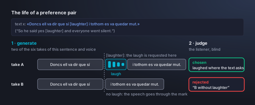
Play the judge: which of the two takes below is the better one?
The text asks for a laugh after «sí». Listen to both and pick the one you prefer.
«Doncs ell va dir que sí [laughter] i tothom es va quedar mut.» “So he said yes [laughter] and everyone went silent.”
Take A
Take B
See what I picked
In the round 1 blind kit, I voted for A and wrote "B without laughter": in A, a short laugh comes in right after «sí»; in B, the sentence goes straight through the tag with no laughter at all. That pair became a training example: A chosen, B rejected.
The DPO formula
Relax, no need to be scared. Now we can look at the math, because you already know what it says. For each pair, the training looks at how much the probability of the chosen take changed relative to the reference model, then does the same with the rejected one and subtracts. That’s the margin. Then it multiplies by a factor β, passes the result through the sigmoid (an S-shaped curve that works as a brake), takes the logarithm, flips the sign and averages over the pairs:

- πθ: the model in training, which keeps changing during the training round at every step.
- πref: the reference model, the frozen snapshot: a copy of the model at the start of the round, which doesn’t change during it.
- yw and yl: the chosen take (winner) and the rejected one (loser) for the same input x, the instruction plus the text.
- β: the factor that multiplies the margin before the sigmoid (and, because of that, what decides how early the brake kicks in). Here,
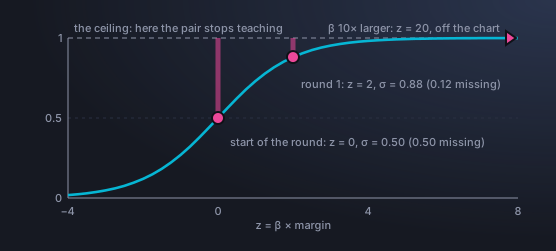
0.01. - σ: the sigmoid, the built-in brake: when margin × β gets large, the curve flattens out and the training stops insisting on that pair.
A pair’s push is β times what’s missing for the sigmoid to reach the ceiling (1). At the start of the round the margin is zero, the sigmoid gives 0.5, and 0.5 is missing. In round 1 the margin got to about 200 (I use 200, which is a round number): 0.01 × 200 = 2, the sigmoid of 2 gives 0.88, and only 0.12 is missing, a quarter of the push at the start. With a β ten times larger the calculation would give 20, and the pair would stop teaching much earlier. Look at the chart:
The two rounds of DPO
In the first round, my focus was to make the model learn to use the laughter tag well. I used 133 best/worst pairs (not counting the ones discarded for being “both bad”), with a recipe of β 0.01, a constant learning rate of 5e-6, and the training objective adds the preference loss to imitation of the chosen take. I got a result of 10 to 3 for the DPO model, and the detected laughter went from 68% to 86%.
In the second round, the focus was something that had been bothering me. It had learned to laugh, but it was common to have a weird pause between the speech and the laughter, as if the speech stopped to wait for the laughter to start. I started from the round 1 model and put together 72 pairs (64 for training and 8 for validation).
A path I parked: reinforcement learning
I also tried reinforcement learning (GSPO, group sequence policy optimization), with the ASR transcribers’ automatic score as the reward. There were three cycles, and all three improved the probe without winning by ear (the third ended up 8 to 8 against the starting point, with 4 ties and 8 “both bad”). If it were a rock show, it would have been an improvement in the details of a guitar solo, but the audience felt zero difference. In other words, the model learned to score well on the probe, which counts correct letters, and the ear judges something else.
Running your model
Training the actor (the llm.pt) is only half of the way. To hear a sentence, you still need the program that runs this model at each request.
Remember the studio with four employees? Missing is the crew working around the actor: the production team, who doesn’t appear in the recording. That’s the synthesis program.
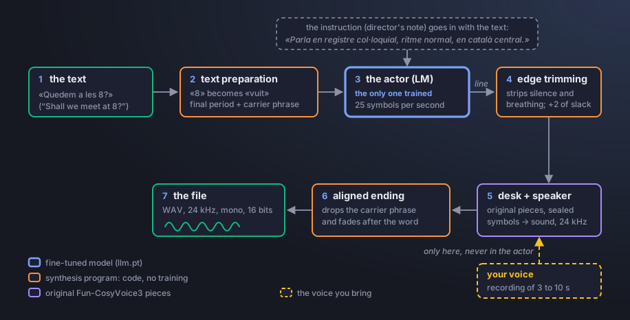
The same path, in pseudocode (the lines with [program] are the production steps): notice where the voice comes in, at the mixing desk (the flow), and nowhere else.
synthesize.py · pseudocode, not the real script
def synthesize(text, ref_wav=None, seed=7):             # real use: the text and the recording (without it, the package's default voice)
    text = prepare_text(text)                           # [program] numbers spelled out; final period; a single word becomes «Mira. hola.»
    tokens = lm.generate(SOS + bpe(INSTRUCT + text) + TASK,
                         seed=seed)                     # the actor: the only step that draws at random
    tokens = trim_edges(tokens)                         # [program] strips silence and breathing from the ends
    tokens = pad_end(tokens)                            # [program] +2 silent symbols at the end: they catch the click
    mel = flow_decoder(tokens,                          # the mixing desk, sealed: the voice comes in HERE, and only here
                       campplus(ref_wav),               # the voice badge
                       s3_tokenizer(ref_wav),           # the annotator: the symbols of the recording itself
                       mel_of(ref_wav))                 # the picture of the sound (the mel) of the recording
    wav = hift_vocoder(mel)                             # the loudspeaker, sealed: picture of the sound -> 24 kHz wave
    return aligned_ending(wav, text)                    # [program] 100 ms fade after the last word
As you can see in the pseudocode comments, we need to prepare the text before sending it to the model. A few things we should pay attention to:
The final period: without it, the actor treats the text as something that’s still going to continue and leaves the last syllable hanging (try saying out loud the sentences “Tomorrow I’m going…” and then “Tomorrow I’m going.” and pay attention only to the last syllable).
Numbers: CosyVoice’s built-in text preparation reads all non-Chinese text as English («a les 8» becomes «a les eight»), so prepare the text beforehand and turn the built-in one off (
text_frontend=False).(Optional) Carrier phrase: a single word is a hard request for a conversational model, because in conversation almost no word lives on its own. In those cases, the program can insert a period, to serve as a valley of silence, and separate the words. Something like: «Mira. hola.» and cut the «Mira.» at the valley between the two words.
The program also trims the silence and breathing from the ends and fades the volume down right after the last word, so as not to leave a pop at the end (the “click”). It’s finishing work, and every piece of it was born from a measured defect.
Running my vermut-tts model
Time to get your hands dirty. The model is on Hugging Face and, to use it, the machine needs very little: 5.4 GB of download and about 5.5 GB of GPU memory at peak (tested on an NVIDIA GB10 GPU, on Linux aarch64, with Python 3.11, CUDA 13.0 and PyTorch 2.14.1; the model card says 2.12 to 2.14 work). A GPU is recommended: I haven’t tested on CPU.
In the terminal (downloads about 5.4 GB, GPU recommended):
# 1. the Hugging Face download tool, and the model folder (5.4 GB)
pip install -U huggingface_hub
hf download fabriciocarraro/vermut-tts --local-dir vermut-tts && cd vermut-tts
# 2. CosyVoice's code, pinned to a commit, unmodified
git clone --recursive https://github.com/QwenAudio/CosyVoice
cd CosyVoice && git checkout 074ca6dc9e80a2f424f1f74b48bdd7d3fea531cc && git submodule update --init --recursive && cd ..
# 3. the libraries: your platform's PyTorch (see pytorch.org) and then the package's list,
#    which is not CosyVoice's list (that one is for training and asks for an older PyTorch)
pip install torch torchaudio
pip install -r requirements.txt
# 4. where Python looks for code
export PYTHONPATH=$PWD/CosyVoice:$PWD/CosyVoice/third_party/Matcha-TTS
# 5. three requests with the package's default voice: a sentence, a sentence with laughter, a single word
python synthesize.py --model-dir . \
  --text "Bon dia! Com estàs?" --out out.wav
python synthesize.py --model-dir . \
  --text "Vinga, va, que t'ho dic de debò. [laughter]" --out laugh.wav
python synthesize.py --model-dir . \
  --text "hola" --out hola.wav
# 6. the same sentence with your voice (3 to 10 seconds of a recording you have the right to use)
python synthesize.py --model-dir . --ref-wav my_voice.wav \
  --text "Bon dia! Com estàs?" --out mine.wav
What runs the package is the requirements.txt that comes in the model folder, tested in a fresh environment (Python 3.11, PyTorch 2.14.1, torchaudio 2.11.0 and the regular onnxruntime), so start from a fresh environment. The block’s pip install torch torchaudio grabs the newest version; if something breaks, go back to the versions I tested, the ones above.
The first three requests I left in that code use the package’s default voice (voices/default.wav, from a volunteer). The last request swaps it for your voice, which should be in my_voice.wav (about 10 seconds of a recording you made yourself). Each command generates a single take (if you didn’t like it, change the --seed, which is set to 7 by default, to another number). The system will run and the model will generate an out.wav audio file.
Congratulations, you just made vermut-tts speak Catalan!
What vermut-tts still gets wrong
These are the boundaries I know of (the model card has the list of known limitations, which includes acronyms):
- The laughter. The short, odd pause before the laugh still shows up. In about one request out of ten the laugh doesn’t come out at all (almost always when you ask for it at the end of the sentence), and sentences that start with laughter sometimes come out with the ending cut off.
- Sounds and melody. «jo» and «ja» sometimes come out with the “y” of “yacht” instead of the “s” of “measure” (4 of 20 pairs in the kit). From 15 to 22% of statements end rising like a question (the corpus itself does that 16.5% of the time). There may be a click at the end of some takes.
Before publishing: the checklist
- License and data: the most restrictive license governs the weights, and pieces under other licenses stay under theirs. A non-anonymized copy of a corpus whose public version was anonymized is a question for whoever is responsible for the data, whatever the license says.
- Voices are people: ask the corpus owner, in writing, what the speakers’ agreement covers, and don’t publish the voice of someone who only consented to research. Either the user brings the voice, or the package ships only the voice of someone who authorized that distribution in writing.
In my case (it’s all in the model card):
- License and data: the weights are released under CC BY-NC-SA 4.0 (for non-commercial use only), and the non-anonymized copy of one of the corpora came in with the agreement of whoever holds the data.
- Voices: the speakers’ agreement for one of the corpora covers non-profit research and teaching, and no speaker in any corpus consented to cloning. That’s why the package doesn’t ship the voice of any of them and the card forbids imitating them. The package’s default voice is from a volunteer who isn’t in any corpus and authorized it in writing.
Audio credits
The real conversation excerpts in this article and the two voices in the examples come from Glissando-ca, a freely distributed corpus available at ELRA (ELRA-S0407) under the Creative Commons license CC BY-NC-SA 3.0 Spain: Garrido, J. M. et al. (2013), “Glissando: a corpus for multidisciplinary prosodic studies in Spanish and Catalan”, Language Resources and Evaluation 47(4), 945-971 (doi:10.1007/s10579-012-9213-0). No speaker is identified, and the permission from the corpus coordinator covers non-profit research and teaching: it doesn’t authorize anyone to clone those voices outside of that.
Next steps
To wrap up, three invitations for anyone who wants to take the recipe and go further (what else I haven’t tested, like CPU and less data, shows up where each thing comes in the text):
- A jury of native speakers (the MOS): native listeners scoring from 1 to 5, blind, with real recordings hidden in the mix. It’s the step vermut-tts still owes: today the one judging is me, alone, and there’s no comparison with other systems.
- More voices from outside the corpus: I tested only one, the package’s default voice.
- Other cuts and other languages: the recipe was only tested on conversational Central Catalan, without Valencian and without formal reading.
To go deeper
- The model: huggingface.co/fabriciocarraro/vermut-tts. The card has samples to listen to without installing anything, the list of known limitations and the data credits.
- CosyVoice’s code (the studio): github.com/QwenAudio/CosyVoice (the old address, FunAudioLLM/CosyVoice, redirects to it), and the CosyVoice 3 technical report (arXiv:2505.17589), which describes the base model and the training with about a million hours.
- DPO: Rafailov et al., 2023, “Direct Preference Optimization: Your Language Model is Secretly a Reward Model” (arXiv:2305.18290).
And that’s pretty much it! :) If I had to sum up the project in a single line: the real cost was deciding what to teach, with which data, and listening A LOT. The whole recipe trains in about 3 hours of H100 GPU, and the entire project used about two weeks of them. A good part of the stumbles along the way came from my process, and the model was hardly to blame.
Happy studying!