Embeddings: The Map That Teaches AI to Understand the World
Published on
You’ve probably never used the word embedding in a normal conversation. Fair enough. It looks like one of those technical terms that lives in documentation and only shows up when someone wants to complicate an explanation.
But I’ll tell you right away that it’s not quite like that, and that if you use AI models like LLMs in your day-to-day, you’re using embeddings.
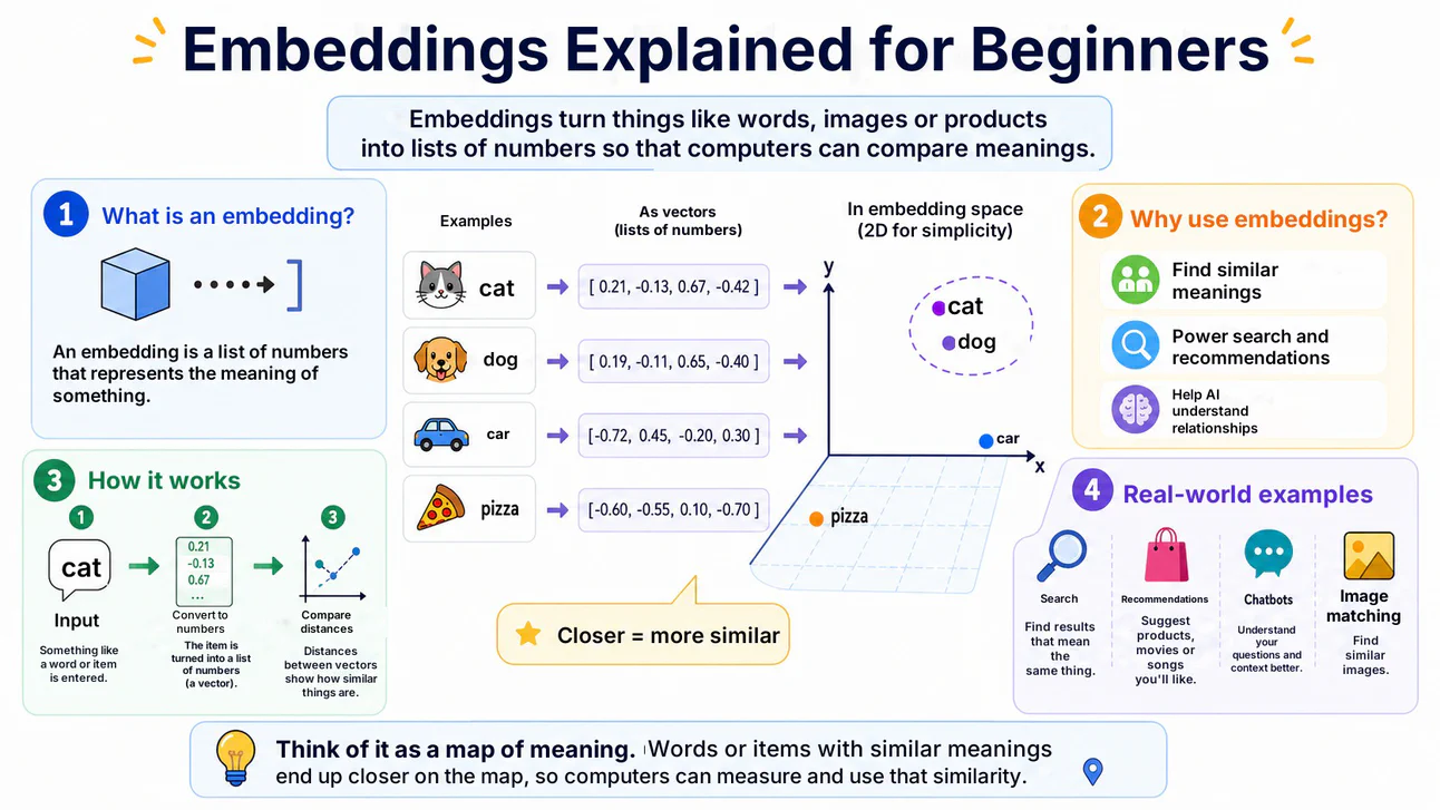
Remember that computers don’t understand words, only numbers, right? Well, the core idea of embeddings is simple: turn things that are hard to compare directly, like texts, images, audio, products or questions, into lists of numbers. And best of all, those lists of numbers manage to create a “mathematical map” of the meaning of each word, sentence or image. On that map, similar things end up close together and different things end up far apart.
That’s what lets a system understand that the questions “how do I cancel my contract?” and “I want to end my subscription” are talking about practically the same thing, even without repeating the same words.
So you could say embeddings are a bridge between the human world of meaning and the mathematical world of machines.
In this article, I’m going to walk you through all of that: what embeddings are, how they work on the inside, how they show up in the training of modern LLMs, and why they matter so much for building a little RAG system.
It’s going to be a bit long, but I promise the trip will be worth it. Shall we?
Computers Can’t Read, They Can Only Count
Before defining embeddings, I need to lay out the problem they solve, because it’s a very concrete one.
A processor, whether in a computer or a GPU training an AI model, understands absolutely nothing about language, meaning, context or intent. It only knows how to do math with numbers. Multiply matrices, add values, apply mathematical functions. That’s it.
So how do you get a computer to understand that the words “dog” and “canine” are synonyms, that “king” is to “queen” what “man” is to “woman”, or that “bank” can mean a financial institution or the side of a river depending on the context?
The naive answer, and one that was widely used until a little over a decade ago, was to create a table where each word gets a number, and that’s it. For example: “dog” = 1, “canine” = 2, “cat” = 3, “airplane” = 4, etc.
But that doesn’t work for anything beyond identifying individual words. The number 1 has no relationship whatsoever with the number 2.
There was also a slightly more sophisticated alternative, one-hot encoding. If your vocabulary has 200,000 words, you create a vector with 200,000 positions full of zeros, with just a single 1 in the position of the word in question. That way, “dog” would become [1, 0, 0, 0, …, 0], “canine” would become [0, 1, 0, 0, …, 0], etc.
The problem is that this doesn’t capture meanings or semantic connections between words either. There’s no way to tell from those numbers that the words “dog” and “canine” have any relationship. From the point of view of what a computer sees, the word “dog” would be just as close in meaning to “canine” as it would be to “airplane” or to “macarena” (the dance craze).
That’s where embeddings come in.
What an Embedding Really Is
“An embedding is a coordinate in a high-dimensional vector space, and the position of that coordinate carries meaning”.
Okay, breathe. Let’s try again, step by step:
An embedding is a vector of numbers, something like [0.82, -0.41, 0.67, …, 0.12]. Better, right?
Moving on: each number in that vector represents a dimension. Those dimensions usually don’t have a human meaning on their own. The meaning shows up in the pattern of the whole vector.
Now, remember math class at school, where we had a graph with the dimensions “x” and “y”?
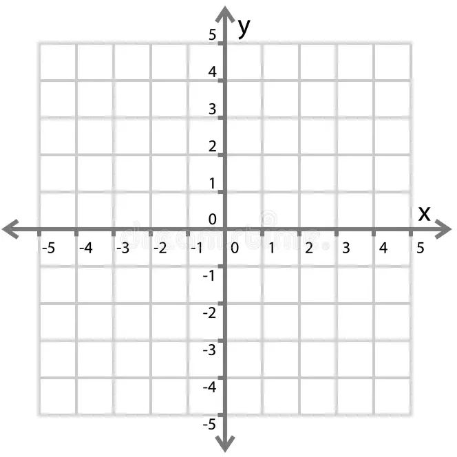
It’s basically the same thing, but instead of being a 2-dimensional graph (“x” and “y”), this graph can have 100, 200, 1,000 or 3,000 dimensions, something we humans can’t really visualize.
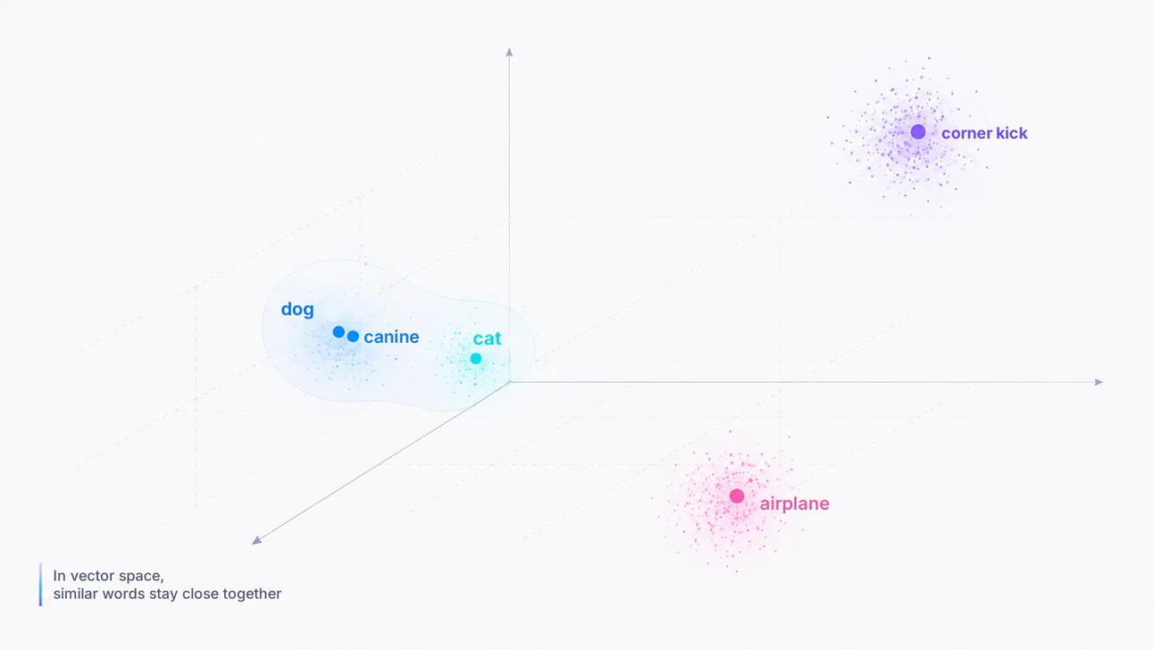
We can consider that each point on this graph will represent a word, like “dog”, “canine” and “airplane”.
But when this “graph” is built (the “high-dimensional vector space” I mentioned in the first sentence of this chapter), it’s done in a way that the position of the point on the graph carries meaning. So you can infer that points that sit close to each other have a similar meaning.
For example, in our embeddings graph (the “high-dimensional vector space”), the point representing the word “dog” would be VERY close to the point representing the word “canine”. And both would be close to the point representing the word “cat”. However, all three of those points would be far away from the point representing the phrase “corner kick”. Did that make sense?
A hypothetical example of what some word embeddings could look like (heavily simplified, with only 4 dimensions, so it fits here):
"dog"         = [0.82, -0.41, 0.67, 0.12]
"canine"      = [0.80, -0.38, 0.65, 0.15]   # very close to "dog"

"cat"         = [0.75, -0.30, 0.58, 0.08]   # close, but not as much

"corner kick" = [-0.20, 0.65, -0.10, 0.90]  # far away

"macarena"    = [-0.50, 0.42, -3.40, -2.90]  # also far away
And that’s it. Two vectors that are close, according to a similarity metric, indicate that the concepts are semantically similar. It’s that simple, and it’s insanely powerful.
Like I said, in practice these vectors have hundreds or even thousands of dimensions. Google’s gemini-embedding-2 model, for example, produces vectors with 3,072 dimensions, not just 4.
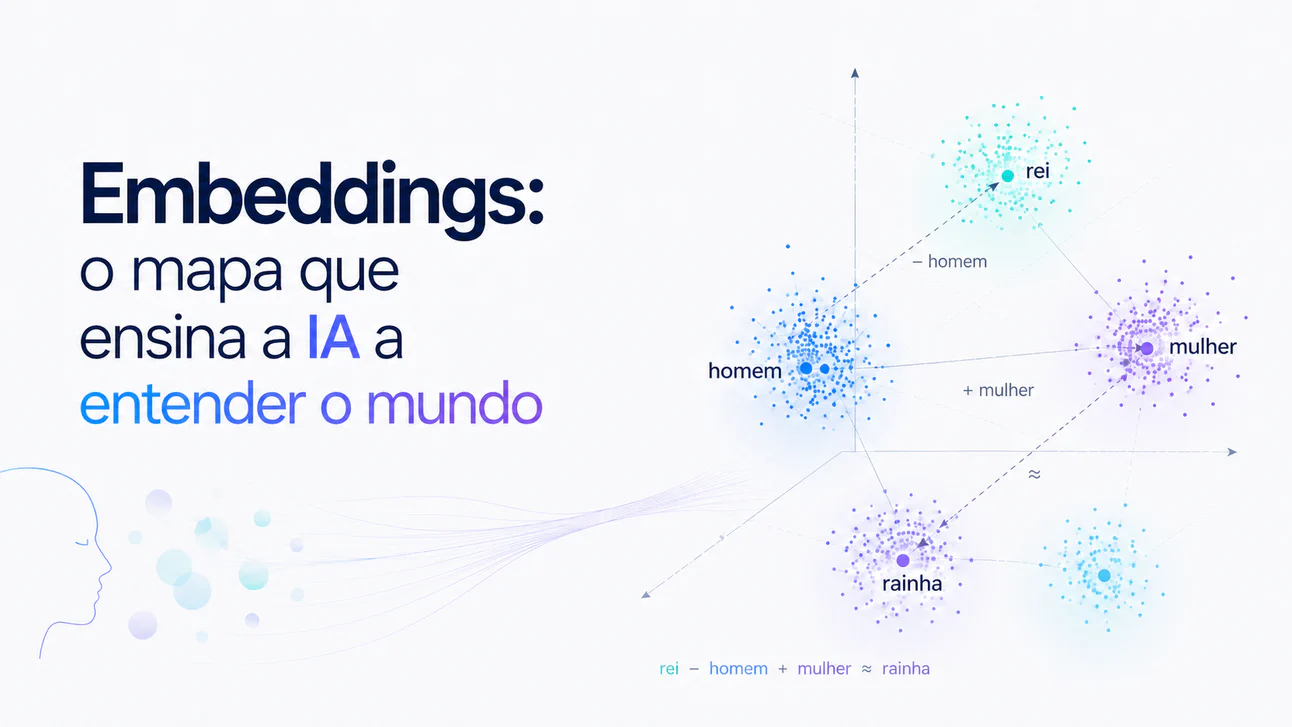
And maybe the most impressive thing of all is that, since they’re vectors, you can do arithmetic with them. The classic example everyone cites, which became famous in 2013 with the Word2Vec work (more specifically in the paper Linguistic Regularities in Continuous Space Word Representations, by Mikolov et al.), is:
embedding("king") - embedding("man") + embedding("woman") ≈ embedding("queen")
Yes, really. You can take the numeric vector that represents the word “king”, subtract from it the numeric vector that represents the word “man”, and add to that the numeric vector that represents the word “woman”, and the result will be very close to the numeric vector that represents the word “queen”.
I know, it’s absurd. But it’s not magic, it’s just a consequence of the fact that the embedding space captures relationships, not just isolated meanings. The vector difference between “king” and “man” seems to capture a recurring relationship in the text corpus that points to the concept of “male royalty”, and when you subtract “man” and add “woman”, you land close to the concept of “female royalty” (also known as “queen”). Wonderful, isn’t it?
The Short History: From Word2Vec to the Transformer
Embeddings weren’t invented yesterday. They have a pretty interesting history, and understanding that history helps you understand WHY modern models work the way they do.
The historical turning point was in 2013, when Tomas Mikolov and his team at Google released Word2Vec. The core idea was to train a shallow neural network to predict, given a word, the words around it (or vice versa). And the result of that task wasn’t the prediction of the words themselves, but rather what was left in the middle of the network after training: the weights of an intermediate layer that ended up capturing incredibly rich semantic relationships. That classic “king” and “queen” example came from there.
Shortly after came GloVe (from Stanford), which took a different approach. Instead of learning word by word from local neighborhoods, it looked at global statistics of how those words appeared near each other across the whole corpus. Oh, and each word had a fixed embedding vector.
And that was exactly the problem. The word “bank” in the sentence “I went to the bank to withdraw money” and in the sentence “I sat on the river bank” generated the SAME vector with Word2Vec and GloVe. The embedding was static, glued to the word, with no regard for the surrounding context.
In 2018, Google released BERT (Bidirectional Encoder Representations from Transformers), and that changed everything. BERT popularized “contextual embeddings”, that is, a word’s vector changes depending on the context it appears in. So the financial “bank” gets a different embedding from the river “bank”, because BERT looks at the whole sentence at once, taking into account the context to the left AND to the right at the same time (hence the “Bidirectional”), before generating the embedding vector for each word. Unlike earlier approaches that made two separate passes (one from left to right, another from right to left) and then merged them, BERT sees the entire sequence simultaneously.
The architecture behind this is the Transformer with its “attention” mechanism, which I already discussed in the article about how AI works, from silicon to chat. With this attention mechanism, each token consults all the other tokens in the sequence to build its own vector, and it’s exactly this process that generates embeddings rich in semantic context.
How Embeddings Enter the Training of Modern LLMs
When a modern LLM (GPT, Claude, Gemini) is trained from scratch, the embeddings are trained together with the neural network itself. They’re initialized randomly and learned along with all the other weights during training.
The flow goes like this:
- All the texts in the dataset that will be used to train the model go through tokenization, which is when words are turned into subwords (for example, a tokenizer could split the word “unhappy” into two tokens: “un” and “happy”). In that process, words become tokens, and those tokens become a sequence of numeric IDs (identifier numbers). Let’s suppose the token “un” has ID 14, and the token “happy” has ID 2845. If the same is done for the word “unable”, it’s possible that it will also be split into two tokens (“un” and “able”), and so the token “un” would have the same ID 14.
- An embedding layer (basically a big table) converts each ID into a dense vector. If the model’s vocabulary has 200,000 tokens (which is a common value in large models) and the embedding dimension is 4,096, this layer would be a matrix of 200,000 × 4,096 parameters that the model keeps adjusting throughout training (careful: don’t confuse the internal dimension of an LLM in training with the output dimension of an embeddings model, like the gemini-embedding-2 I mentioned earlier).
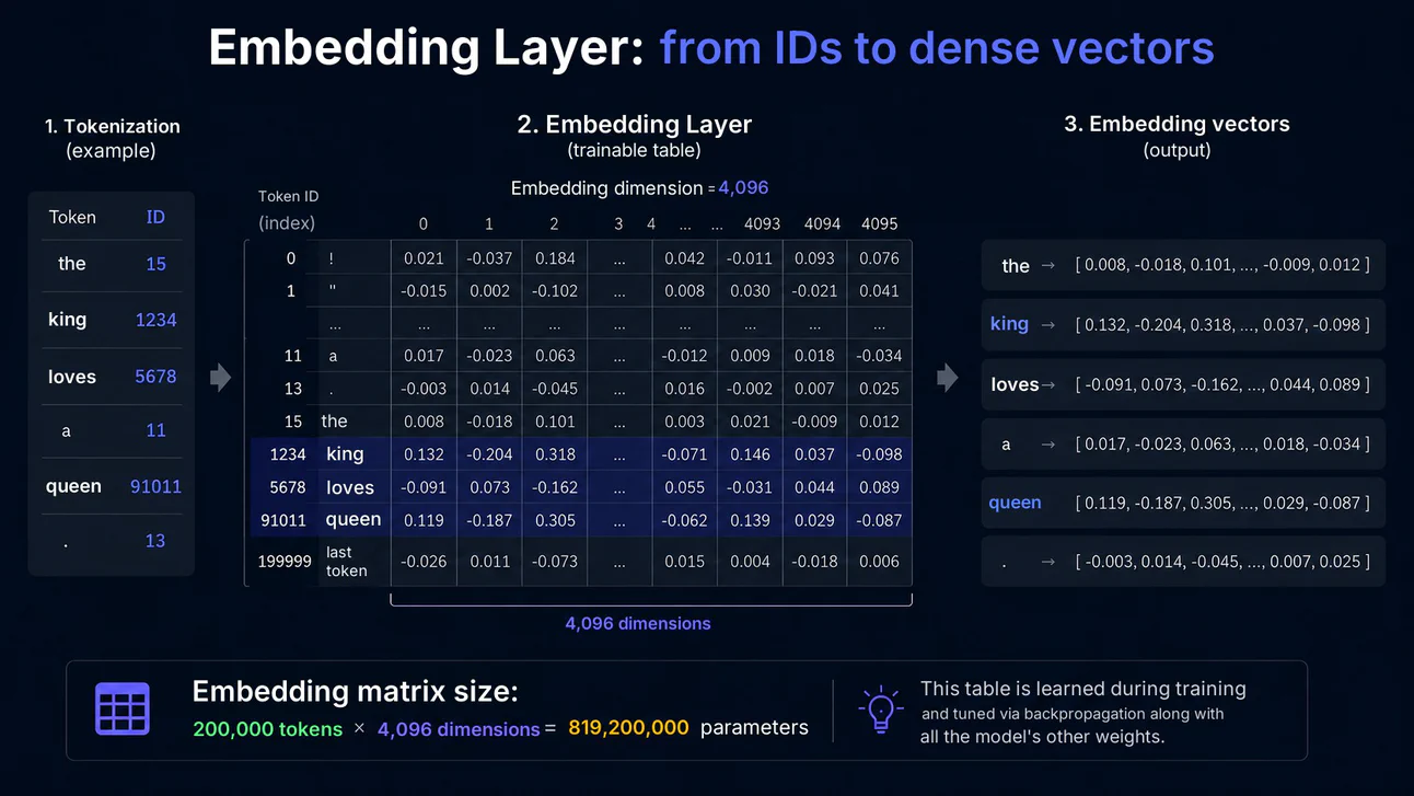
- The model also needs to know the position of each token in the sequence. Think of an attendance list that notes not only who is in the room, but which chair each person is sitting in. Without that information, the sentences “The dog bit the man” and “The man bit the dog” would be indistinguishable to the model, since the same words in a different order would generate exactly the same input. Historically this was done by adding a positional embedding (a position vector) to the token’s embedding. The most modern LLMs tend to use smarter variants, like RoPE (Rotary Position Embeddings), which encodes the position inside the attention mechanism instead of adding a vector at the input. But the core idea is the same: give the model a sense of order.
- Those vectors, together with some positional information mechanism, enter the attention and feedforward blocks of the Transformer (the LLM’s architecture).
- Across the layers, the vectors keep getting refined. What came in as a static, context-free embedding of the token “bank” (the same vector, regardless of the sentence) comes out of the last layer as a very rich numeric vector that manages to capture that this vector refers to the “bank where I’m going to withdraw money” or to the “bank of a river”.
The key point is that embeddings are learned, they’re not fixed. They start out random and get adjusted by the LLM neural network’s backpropagation the same way as all the other weights in the network. By the end of training, they end up capturing semantic relationships because the model discovered that having similar words close to each other in the vector space helps it solve the training task better (predicting the next token, in the case of generative LLMs).
Nobody told the model “put ‘dog’ and ‘canine’ close together”. It learned that on its own because it made statistical sense given the training data.
Measuring Distance Between Embeddings: How AI Knows What’s Similar
Great, we have the vectors. But how do we turn close vectors into something computationally useful?
The most widely used metric for text embeddings is cosine similarity. Instead of measuring the standard distance (also called “Euclidean”) between two points, which can be fooled by the size of the vectors, cosine similarity measures the angle between the two vectors. Two vectors pointing in the same direction have a cosine similarity of 1.0 (identical). Perpendicular vectors have a similarity of 0.0, which indicates a neutral or weak similarity. Vectors in opposite directions have a similarity of -1.0, which means they’re maximally misaligned in that vector space.
In the context of text embeddings, it’s important to be careful with this interpretation: -1.0 doesn’t necessarily mean that two words are “opposites” in the human sense, like “happy” and “sad”. It only means that, mathematically, the vectors point in opposite directions in that space.
What matters for semantics isn’t how “big” a word’s vector is, but which direction in space it points to. That’s why, in textual semantic search, it’s very common to use cosine similarity or the inner product with normalized vectors (although Euclidean distance also shows up in some systems).
Two texts with the same meaning will very likely point in the same direction, even if one is longer than the other. Example:
# hypothetical numbers, just to illustrate

cosine_similarity("dog", "canine") = 0.98          # very similar
cosine_similarity("dog", "corner kick") = 0.32     # very different
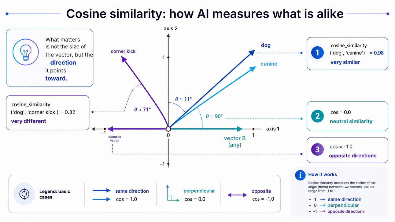
There are other metrics that can be used, but in most semantic search cases, cosine similarity is the most common choice, precisely because it looks at the direction of the vectors, not their size.
RAG: Where Embeddings and LLMs Truly Meet
Now we get to one of the most important and practical applications of embeddings: RAG (Retrieval-Augmented Generation).
When you train an LLM, you use huge datasets. But how is the model going to know what the score of the Brazil game was yesterday if the most recent data used to train it is 6 months old? The raw model, without internet search tools, has no way of knowing anything that happened after that date. On top of that, the model doesn’t know your company’s internal documents, your legal team’s PDFs, your HR’s latest policies or the documentation of the API you maintain.
To solve that, one possible solution would be fine-tuning, retraining the model with that data, but that’s pretty expensive, slow and hard to keep updated (if the PDF changes, you’d have to retrain the model to make it “forget” the old information and “learn” the new one).
That’s why RAG is a much more practical alternative. Instead of trying to teach the model that internal information (which it might even hallucinate when generating an answer, if the training wasn’t ideal, or the temperature is high, or a number of other factors), you simply do a quick internal search in your documents, hand the result of that search to the model, and ask the model to generate a nice, formatted answer. And embeddings are the central piece that makes that search possible.
This process has two very distinct moments:
Moment 1: indexing (happens before the search)
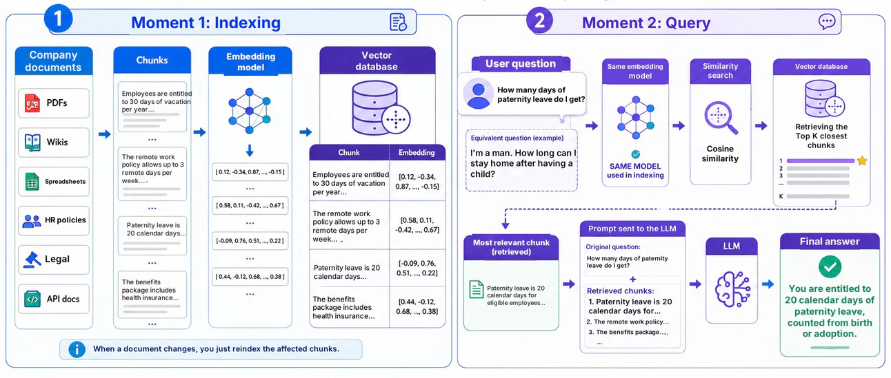
You take all of your company’s documents (PDFs, wikis, spreadsheets, whatever), break them into smaller pieces called chunks, and run each chunk through an embedding model. That way, each chunk is turned into a numeric embedding vector that captures the semantic meaning of that piece. Those vectors are stored in a table in a vector database, along with the chunk’s original text. For example, something like:
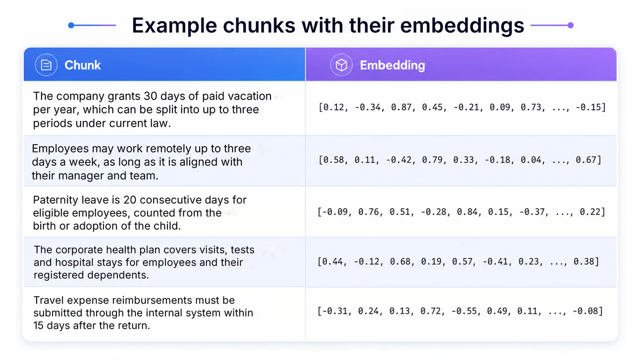
If a document has a piece changed in the future, you just generate the embedding vector for the new chunk and update the vector database. The same goes if you want to add or delete a document.
Moment 2: query (happens with every question)
- The user asks a question.
- That question goes through the same embedding model that was used in indexing (this is KEY, the vector spaces need to be compatible), and also becomes an embedding vector, which captures the semantic representation of that question.
- The vector database runs a search, usually using cosine similarity, to try to find the chunks whose embedding vectors are closest to the question’s.
- It returns a number K of chunks (we can set the value of “K”), ordered from closest to farthest.
- The original text chunks matching those vectors are retrieved from the table and placed in the LLM’s prompt, along with the original question.
- The LLM answers based on the real information that was retrieved and handed to it, not on what it “thinks it knows”.
The beauty of this is that it works semantically, not by keywords. Imagine two example questions:
- “How many days of paternity leave do I get?”
- “I’m a man. How long can I stay home after having a child?”
Even though the words used in the questions are completely different, you’ll agree they mean practically the same thing, right?
A simple keyword search system wouldn’t find anything for the second question. An embeddings-based system does, because the numeric vectors of the two sentences are close together in the semantic space.
A Practical Example in Python
Using the sentence-transformers library (free, runs locally) and Microsoft’s microsoft/harrier-oss-v1-0.6b model, you can put together a minimal RAG system in very few lines. This model is part of the “Harrier-OSS-v1” family, an open-source family of multilingual embedding models. The 0.6b version has about 0.6 billion parameters and produces 1,024-dimensional vectors, which is really interesting if you work with languages other than English:
from sentence_transformers import SentenceTransformer
import numpy as np

# Loads the embedding model
model = SentenceTransformer("microsoft/harrier-oss-v1-0.6b")

# Simulates a document base (chunks)
documentos = [
    "The benefits package includes health insurance and meal vouchers.",
    "Employees are entitled to 30 days of vacation per year.",
    "The remote work policy allows up to 3 remote days per week.",
    "The hiring process takes about two weeks on average.",
    "The company offers an education allowance of up to $800 per month.",
]

# Generates embeddings for the documents (indexing)
embeddings_docs = model.encode(documentos)

# User's question. Harrier is instruction-tuned: the query carries a task
# instruction (passed via prompt=), while documents are encoded without one
instrucao = "Instruct: Retrieve the passage that answers the question\nQuery: "
pergunta = "what are the employee benefits?"
embedding_pergunta = model.encode([pergunta], prompt=instrucao)

# Computes cosine similarity against all the chunks
from sklearn.metrics.pairwise import cosine_similarity

scores = cosine_similarity(embedding_pergunta, embeddings_docs)[0]

# Retrieves the most relevant chunk
idx_melhor = np.argmax(scores)

print(f"Most relevant chunk (score {scores[idx_melhor]:.3f}):")
print(documentos[idx_melhor])

# → "The benefits package includes health insurance and meal vouchers."
This is the skeleton of any RAG system. In production, “embeddings_docs” would live in a dedicated vector database instead of a Python list, and the retrieved chunk would be sent to an LLM to generate the final answer. But the logic is exactly this.
Choosing the Right Embedding Model for RAG
A common mistake is thinking that “any embedding will do”. It won’t. The choice of embedding model directly affects the quality of the search, which directly affects the quality of the LLM’s answers.
To navigate this sea of options, there’s the MTEB Leaderboard (Massive Text Embedding Benchmark), maintained on Hugging Face, which evaluates embedding models on several tasks: retrieval, semantic similarity, classification, clustering, multiple languages, etc.
A few practical considerations when choosing:
- Vector dimensions: more dimensions (like the 3,072 of gemini-embedding-2) can give more capacity to capture nuance, but they don’t guarantee a better result. Quality depends a lot on the training, the domain and the task. Larger dimensions also increase storage and search costs. For many cases, 384 or 768 dimensions are more than enough.
- Paid vs. open-source models: Google’s gemini-embedding-2 and OpenAI’s text-embedding-3-large are excellent and easy to use via API, but they charge per token. Models like jinaai/jina-embeddings-v5-text-small or microsoft/harrier-oss-v1-0.6b, on the other hand, can be run locally on your laptop, are free and are enough for many cases. Just keep an eye on the license: Jina v5 is CC BY-NC 4.0 (non-commercial use, commercial use needs a separate license), while harrier-oss is MIT (cleared for commercial use). For RAG inside a company, that makes a difference.
- Multilingual: if your system needs to understand text in multiple languages, use a multilingual model explicitly trained for that. A model trained only in English or with little data in other languages will work very poorly for those other languages.
- Specific domain: generic models may not work well in very technical domains (medical, legal, code). Sometimes it makes sense to fine-tune an embedding model with data from your domain.
One important note: the embedding model used for indexing and the model used for the query MUST be the same. If you indexed with text-embedding-3-large and tried to search with gemini-embedding-2, you’ll get completely meaningless results, because they’re incompatible vector spaces.
Beyond Text: Multimodal Embeddings
So far I’ve only talked about text, but embeddings exist for practically any kind of data. Images, audio, video, code, molecules… anything a neural network can process can be mapped into a vector space.
The most famous example of a multimodal embedding is CLIP (Contrastive Language-Image Pretraining), from OpenAI. CLIP trained two encoders, one for text and one for images, to put text and images in the same vector space. With that, you can send the text “a dog running on a beach at night”, and the system can return images that semantically match the description, without depending on tags or manual metadata on the image.
Think about what that makes possible: the vector of a photo of a golden retriever on the sand sits mathematically close to the vector of the sentence “dog on the beach”. They’re completely different modalities, but they exist and work in the same space of meaning.
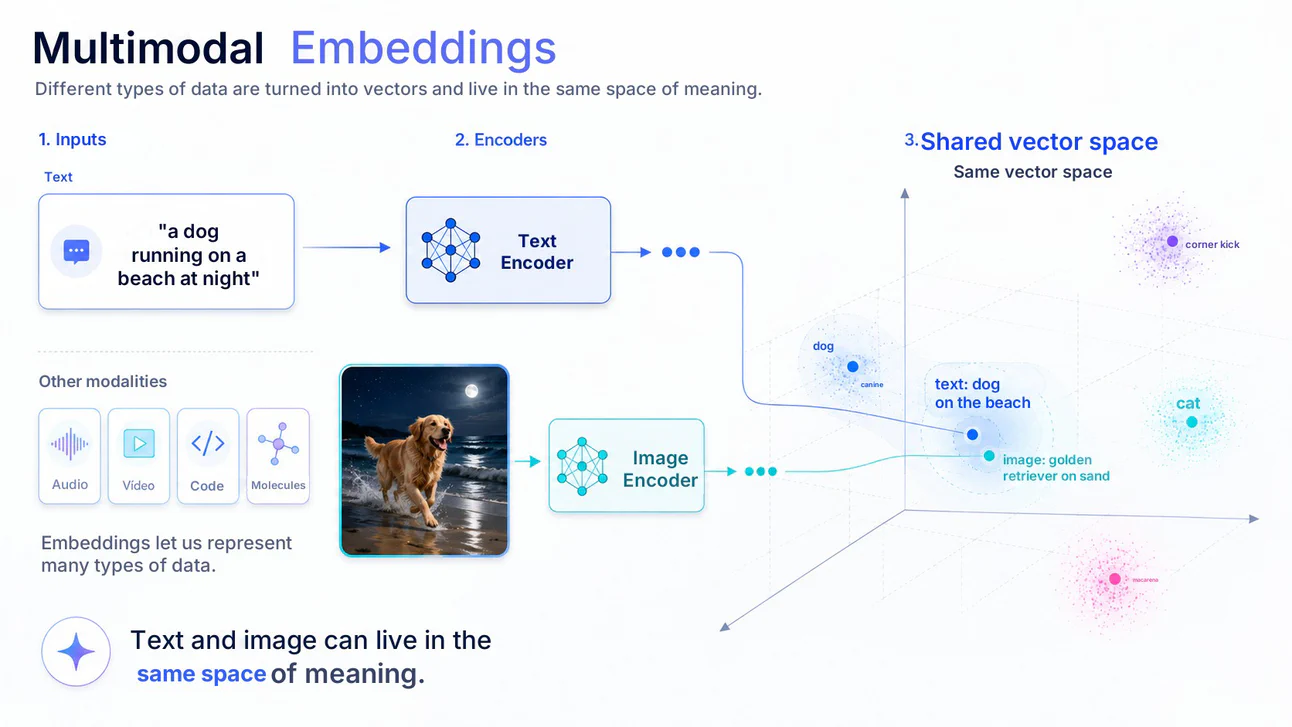
If you want to see this working in practice, Pedro Gengo and I created a complete guide to Gemini Embedding 2, Google’s first natively multimodal embeddings model. In the Google Colab notebook, we show step by step how to generate and compare embeddings of text, images, audio, video and PDFs, as well as run searches across different modalities, like using an image to find an audio clip or a voice recording to search a PDF. Everything runs in a single Colab and you can run the examples on your own.
Conclusion
At the end of the day, embeddings are one of those ideas that seem scary the first time they show up, but get a lot friendlier once you realize what they actually do, which is translate, for a computer that only understands numbers, the complex contextual and semantic meanings of human language.
The computer still doesn’t “understand” the world the way we do. It doesn’t know what a dog, a queen or an overdue bill on a Monday morning is. But with embeddings, it can organize those concepts in a way that’s useful enough to find relationships, compare meanings and help AI models answer better.
In other words: embeddings aren’t just vectors full of strange numbers. They’re the map that helps AI find its place in the world of meaning.
Happy studying!